1
Resampling and Reconstruction with Fractal Interpolation Functions Jeffery R. Price, Student Member, IEEE and Monson H. Hayes III, Fellow, IEEE Abstract— An alternative form of the fractal interpolation function (FIF) – previously unmentioned in the signal processing literature – is noted. This form highlights a simple relationship between fractal and linear interpolation. Using this relationship, many FIF problems can be reduced to a matrix/vector expression. This expression provides a more powerful way to employ the FIF for interpolation and permits its adaptation for reconstruction. Additionally, the alternate form of the FIF allows the construction of fractal functions whose piecewise integrals match observed data.
1
D
g1 = 0.4
g2 = 0.6
g3 = 0.3
D1
D2
D3
0
Keywords— Fractal interpolation, reconstruction.
I. Introduction and Review
F
RACTAL interpolation, first described in [1], has been used for various data visualization and modeling problems [2]-[7]. In this letter we describe a form of the FIF which simplifies its implementation and allows it to be used for reconstruction. In this first section we briefly review the classical form of the FIF as it appears in previous signal processing literature. We then present an alternate form detailed in [1] but largely ignored since. In Section II we describe how this alternate form leads to a matrix/vector expression for many FIF problems and suggest how this expression can be exploited for reconstruction. In Section III we describe how the alternate form also permits reconstruction of a continuous function when the observed data represents its piecewise integrals. A simple example of these reconstructions is given in Section IV. In Section V we make some closing comments. For uniformly sampled signals, we begin with a data set ª © (1) (xn , yn ) ∈ D × R : n ∈ [0, 1, . . . , N ] , where D = [0, 1] and xn = n/N . A continuous function f : D → R is sought that interpolates the data according to f (xn ) = yn
for n ∈ [0, 1, . . . , N ].
(2)
Following the standard form used in the signal processing literature, FIFs are constructed using N affine mappings of the form µ ¶ µ ¶µ ¶ µ ¶ x an 0 x c = + n wn dn bn γn y y for n = 1, . . . , N
(3)
c °1998 IEEE. In IEEE Signal Processing Letters, vol. 5, no. 9, pp. 228-230, September, 1998. The authors are with the Center for Signal & Image Processing, School of Electrical & Computer Engineering, Georgia Institute of Technology, Atlanta, GA 30332-0250 USA (e-mail:
[email protected]). J. Price is a Kodak Fellow.
-1
1/3
0
2/3
1
Fig. 1. Example fractal interpolation function with N = 3.
with subinterval endpoint constraints µ wn
x0 y0
µ =
xn−1 yn−1
µ and wn
xN yN
µ =
xn yn
for n = 1, . . . , N. (4) Equations (3) and (4) imply that each map wn horizontally “shrinks” (by a factor of an ) and vertically scales (by a factor γn ) the entire function over the interval D and maps it to the piece of the function over the interval Dn = [xn−1 , xn ]. (See Fig. 1.) For these mappings to be contractive, it is necessary that |an | < 1 and |γn | < 1. With each γn (referred to as contraction factors) considered a (fixed) free parameter, |an | < 1 is guaranteed by the constraints of Equation (4). The contraction factors, however, must be chosen to satisfy |γn | < 1. Under these conditions the collection of mappings defines a hyperbolic iterated function system whose attractor set in R2 is the graph of a continuous function satisfying Equation (2). An equivalent form for the FIF associated with Equations (1)-(4) is described in [1]. It can be expressed as ¡ ¢ (5a) wn (x, y) = Ln (x), Fn (x, y) Ln (x) = an x + cn (5b) ¡ ¢ (5c) Fn (x, y) = h(Ln (x)) + γn f (x) − b(x) where the height function h(x) is the linear interpolation of the data while the base function b(x) is the linear function through (x0 , y0 ) and (xN , yN ). (More general functions h(x) and b(x) are allowed so long as h(x) passes through each of the data points, b(x) passes through the first and last data points and both are continuous.) In this alternate
2
form, the subinterval endpoint constraints become Ln (x0 ) = xn−1 Fn (x0 , y0 ) = yn−1
and Ln (xN ) = xn (6) and Fn (xN , yN ) = yn . ¡ ¢ Examining Equation (5) we note that Fn (x, y) = f Ln (x) and hence ¢ ¡ −1 ¢¤ £ ¡ f (x) = h(x) + γn f L−1 n (x) − b Ln (x) for x ∈ Dn (7) which is the key expression used in the next sections. In the case of uniform sampling on D = [0, 1] we have an = 1/N and Equation (5b) becomes 1 1 x + (n − 1). N N II. Reconstruction by Interpolation Ln (x) =
(8)
Many interpolation and reconstruction problems can be summarized as follows. Given an (N + 1)-point signal yn , construct an (M + 1)-point signal fn (where M > N ) that is consistent with yn according to some model. For basic interpolation, the model states that yn represents actual points on some continuous function f (x) and fn is a finer sampling of this function. In reconstruction, the signal yn often represents the observation of a higher-resolution signal fn that has been distorted and downsampled. (The effects of noise are not considered in this letter.) We begin with an (N + 1)-point signal yn and seek a signal fn which has P new points inserted between every sample of yn . This corresponds to upsampling by a factor of U = (P + 1). The interpolated signal fn will then have (M + 1) = (N + 1) + N P total points. Although there are various methods [5] to compute points of an FIF, we are interested in only N P specific points. Assuming certain relationships between N and U (to be described shortly), we can use Equation (7) to write ¡ ¢ (9a) fnU +k = hnU +k + γn yl(k) − bl(k) N (9b) l(k) = k U where n ∈ [0, 1, . . . , N − 1] and k ∈ [0, 1, . . . , P ] (which excludes the very last point fM +1 = yN +1 ). The l(k) term is derived from the inverse of Ln (x) in Equation (8) and describes how points of the entire signal propagate to points of each subinterval. We have assumed that N and U are such that l(k) is indeed an integer in [0, 1, . . . , N ]. This can easily be ensured by signal extension or application of the process to pieces of the signal. The bl(k) term represents (N + 1) samples of the base function while hnL+k indicates (M + 1) samples of the height function. We now envision vectors f , h ∈ RM +1 and γ ∈ RN . Letting qk = yl(k) −bl(k) we create a matrix Q ∈ R(M +1)×N q q .. Q= (10) . q 0
¡ ¢T where q = 0 q1 q2 . . . qP so that we can express the FIF problem of Equation (9) simply as f = h + Qγ.
(11)
For interpolation purposes γ is arbitrary so long as |γn | < 1. In many cases, however, we might be interested in choosing γ so that f satisfies some properties. For instance, in speech interpolation it might be prudent to make the relationship between f and h as close to linear phase as possible. For signals that are known to exhibit certain fractal properties, we might try to maintain some estimated fractal dimension as in [2]. These are, in essence, reconstruction problems. A more common reconstruction problem can be stated as follows. Suppose y is a low-resolution observation of a higher-resolution signal z ∈ RM +1 . A known system model implies that y and z are related linearly by y = Az where A ∈ R(N +1)×(M +1) represents some (FIR) distortion and downsampling. For this underdetermined problem an estiˆ is sought so that ky − Aˆ mate z zk is minimized. Referring ˆ = f and let h be some initial esto Equation (11) we let z timate of z. (The base function implicit in the matrix Q is defined by the first and last points of h.) We then seek γ to minimize ky − Af k. The resulting signal f (an approximation of z) is composed of samples of some fractal function. Note that Equation (11) provides a simple expression that can facilitate the selection of γ. Note also that h(x) is arbitrary in this problem so h can be refined if desired. An example of this approach is given in Section IV. III. Reconstruction by Integration In some reconstruction problems the observed data yn might represent the piecewise integrals of an unknown continuous function [8], [9]. In other words, f (x) is sought such R that yn = Dn f (x) dx where now n ∈ [1, . . . , N ]. Applying Equation (7) we can construct such a fractal function. We can then either produce actual points of the resulting function as described previously or integrate over smaller intervals in order to implement resampling. Simplifying the work in [1] for our purposes, we use Equation (7) to write Z f (x) dx yn = Dn Z ³ ¢ ¡ −1 ¢´ ¡ (x) − b Ln (x) dx f L−1 = γn (12) n Dn Z h(x) dx. + Dn
R
¯n = Letting h yields
Dn
h(x) dx and substituting variables Z
¯ n + γn an yn = h Next we let F¯ =
D
¡
¢ f (u) − b(u) du.
(13)
R ¯= f (u)du and B b(u)du which gives D ¡ ¢ ¯ n + an F¯ − B ¯ γn . (14) yn = h
R
D
3
signal z was filtered by a 5-point FIR filter and then downsampled by a factor of 4 yielding the 65-point observation y. For the interpolation-based reconstruction – referring to Equation (11) – we seek γ so that Af ≈ y or equivalently
ORIGINAL
OBSERVATION
AQγ ≈ y − Ah.
INTERPOLATION
INTEGRATION
0
1/4
1/2
3/4
1
Fig. 2. Fractal reconstruction examples.
We choose h(x) and b(x) so that h(x) is some (again arbitrary) initial guess at f (x) while b(x) must satisfy PN b(0) = h(0) and b(1) = h(1). Since F¯ = n=1 yn and an = 1/N , only the contraction factor γn of Equation (14) is unknown. Since it is required that |γn | < 1 a direct solution of Equation (14) might seem infeasible, perhaps implying a constrained optimization approach is necessary. There is, however, an easier method. First solve Equation (14) for γn . If this yields |γn | > 1 then adjust h(x) over Dn so that the solution of Equation (14) does yield |γn | < 1. For example, we might begin with h(x) a piecewise linear function and change it to an appropriate quadratic over Dn if necessary. (This is the approach used in Section IV.) The result is a function f (x) which satisfies R yn = Dn f (x) dx. To resample f (x) by integration we split each Dn into P equal subintervals Dnk for k ∈ [1, . . . , P ] and then compute the N P new integrals of f (x) over these smaller intervals. Assuming N/P is an integer, an expression similar to Equation (14) can be derived: ¡ ¢ ¯ k + an F¯ k − B ¯ k γn (15) ynk = h n for n ∈ [1, . . . , N ] and k ∈ [1, . . . , P ]. In Equation (15), ¯ k are the integrals of f (x) and h(x) over Dk , reynk and h n n spectively. Letting Dk represent the splitting of the entire ¯ k indicate the indomain D into P subintervals, F¯ k and B tegrals of f (x) and b(x) over Dk , respectively. Note that F¯ k can be computed by summing the appropriate (and known) piecewise integrals yn . Note also that it might be desirable to scale the new samples since they correspond to integration over smaller intervals. This will ensure that they are similar in scale to the original data. An example of this approach is given in the next section. IV. Examples We now employ the reconstruction methods of Sections II and III in order to upsample a short segment of a speech signal by a factor of 4. The original 257-point
(16)
Since h can be refined , γ can easily be found so that Equation (16) is equality. The basic idea is to introduce an artificial contraction factor γN +1 and add an extra column to Q so that the matrix product AQ is invertible. Then Equation (16) can be solved for γ. The contributions to f from the artificial γN +1 and any contraction factor for which |γn | > 1 are absorbed into h. The “INTERPOLATION” reconstruction of Fig. 2 was found in this fashion and therefore has zero reconstruction error – i.e., Af = y. For the integration-based reconstruction the first 64 points of y were taken to be the piecewise integrals of some unknown function f (x). This function was found as described in Section III. The reconstruction error here is zero R as well since Dn f (x) dx = yn by construction. The function was then integrated over quarter-intervals and the result scaled by 4 to produce the “INTEGRATION” plot shown in Fig.2. V. Concluding Remarks In this letter we have noted an alternate form of the FIF and shown how it can be applied to reconstruction problems. Although only modest examples were given, the simplicity of the approaches described should permit a wide variety of fractal reconstructions. References [1] M.F. Barnsley, “Fractal functions and interpolation,” Constructive Approximation, vol. 2, pp. 303–329, 1986. [2] Petros Maragos, “Fractal aspects of speech signals: Dimension and interpolation,” in Proc. ICASSP, 1991, vol. 1, pp. 417–420. [3] David S. Mazel and Monson H. Hayes III, “Using iterated function systems to model discrete sequences,” IEEE Trans. Signal Processing, vol. 40, no. 7, pp. 1724–1734, 1992. [4] X. Zhu, B. Cheng, and D.M. Titterington, “Fractal model of a one-dimensional discrete signal and its implementation,” IEE Proc.: Vision, Image and Signal Processing, vol. 141, no. 5, pp. 318–324, 1994. [5] Michael F. Barnsley, Fractals Everywhere, Academic Press Professional, 1993. [6] Craig M. Wittenbrink, “IFS fractal interpolation for 2D and 3D visualization,” in Proc. IEEE Visualization Conference, 1995, pp. 77–84. [7] Nailiang Zhao, “Construction and application of fractal interpolation surfaces,” The Visual Computer, vol. 12, no. 3, pp. 132–146, 1996. [8] Terrance E. Boult and George Wolberg, “Local image reconstruction and subpixel restoration algorithms,” CVGIP: Graphical Models and Image Processing, vol. 55, no. 1, pp. 63–77, 1993. [9] Ming-Chao Chiang and Terrance E. Boult, “The integrating resampler and efficient image warping,” in Proc. ARPA Image Understanding Workshop, 1996, pp. 843–849.