Abstract This paper considers a family of metrics to com- pare images based on their local descriptors. It encompasses the VLAD descriptor and matching ...
Noname manuscript No. (will be inserted by the editor)
Image search with selective match kernels: aggregation across single and multiple images Giorgos Tolias · Yannis Avrithis · Herv´e J´egou INRIA NTUA INRIA
the date of receipt and acceptance should be inserted later
Abstract This paper considers a family of metrics to compare images based on their local descriptors. It encompasses the VLAD descriptor and matching techniques such as Hamming Embedding. Making the bridge between these approaches leads us to propose a match kernel that takes the best of existing techniques by combining an aggregation procedure with a selective match kernel. The representation underpinning this kernel is approximated, providing a large scale image search both precise and scalable, as shown by our experiments on several benchmarks. We show that the same aggregation procedure, originally applied per image, can effectively operate on groups of similar features found across multiple images. This method implicitly performs feature set augmentation, while enjoying savings in memory requirements at the same time. Finally, the proposed method is shown effective for place recognition, outperforming state of the art methods on a large scale landmark recognition benchmark.
1 Introduction This paper is interested in improving visual recognition of objects, locations and scenes. The best existing approaches rely on local descriptors [28, 29]. Most of them inherit from the seminal Bag-of-Words (BOW) representation [42,11]. It employs a visual vocabulary to quantize a set of local descriptors and to produce a single vector that represents the image. This offers several desirable properties. For image classification [11], it is compatible with powerful machine learning techniques such as support vectors machines. In this case, it is usually employed with relatively small visual This work was supported by ERC grant V IAMASS no. 336054 and ANR project Fire-ID. Address(es) of author(s) should be given
vocabularies. In a query by content scenario [42], which is the focus of our paper, large vocabularies make the search efficient [31, 36, 30], thanks to inverted file structures [39] that exploit the sparsity of the representation. The methods relying on these ingredients are typically able to search in millions of images in a few seconds or less. Several researchers have built upon this approach to design better retrieval systems. In particular, the search is advantageously refined by re-ranking approaches, which operate on an initial short-list of images. This is done by exploiting additional geometrical information [36, 32, 44] or applying query expansion techniques [10, 46]. Another important improvement is obtained by reducing the quantization noise. This is done by multiple assignment [37, 20], or by exploiting a more precise representation of the individual local descriptors, such as binary codes in the so-called Hamming Embedding (HE) method [20], or by integrating some information about the neighborhood of the descriptor [51]. All these approaches implicitly rely on approximate pair-wise matching of the query descriptors with those of the database images. In a concurrent effort to scale to even larger databases, recent encoding techniques such as Fisher kernels [33, 35], local linear coding [50] or the “vector of locally aggregated descriptors” (VLAD) [22], depart from the BOW framework by introducing alternative encoding schemes. By compressing the resulting vector representation [22, 34], the local descriptors are not considered individually. Images can be represented by a small number of bytes, similar to coded global descriptors [48], but with the advantage of preserving some key properties inherited from local descriptors, such as rotation and scale invariance. Our paper introduces a framework to bridge the gap between the “matching-based” approaches, such as HE, and the recent aggregated representations, in particular VLAD. For this purpose, we introduce in Section 3 a class of match
2
kernels that includes both matching-based and aggregated methods for unsupervised image search. We then discuss and analyze in Section 4 two key differences between matching-based and aggregated approaches. First, we consider the selectivity of the matching function, i.e. , the property that a correspondence established between two patches contributes to the image-level similarity only if the confidence is high enough. It is explicitly exploited in matching-based approaches only. Second, the aggregation (or pooling) operator used in BoW, VLAD or in the Fisher vector, is not considered in pure matching approaches such as HE. We show that it is worth doing it even in matching-based approaches, and discuss its relationship with other methods (e.g. , [19, 35]) introduced to handle the non-iid statistical behavior of local descriptors, also called the burstiness phenomenon [19]. This leads us to the conclusion that none of the existing schemes combines the best ingredients required to achieve the best possible image retrieval quality. As a result, we introduce a new method that exploits the best of both worlds to produce a strong image representation and its corresponding kernel between images. It combines an aggregation scheme with a selective kernel. This vector representation is advantageously compressed by vector binarization to drastically reduce the memory requirements, while also improving the search efficiency. The compressed vectors offer an efficient way to detect groups of similar features in large image collections. We thus show that descriptor aggregation can further be applied off-line across multiple images. In contrast to previous approaches of feature augmentation [1] or cross matching images for query expansion [12, 41, 14], this method does not increase either storage requirements or query time. Generic image search methods have been shown quite effective for the task of image geo-localization [47]. Location recognition is typically achieved by matching rigid objects, especially buildings. Our approach, by enforcing selective feature matching and by handling burstiness, is successfully utilized for this task. It is true that bursty matches dominate in urban sceneries and building photos. Section 6 shows that our method significantly outperforms the state of the art in a comparable setup, i.e. when comparing the quality of the initial result set produced while searching a large collection. We further evaluate our method on the San Francisco landmark recognition dataset [8], again outperforming the state of the art. This paper is the continuation of our previous work [45]. In the original work we presented the common framework for matches kernels and the selective match kernels for single images, now described in Sections 3 and 4, respectively. The new contributions are the extension to aggregation of similar features derived from multiple images, described in Section 5, and the application on place recognition.
Giorgos Tolias et al.
2 Related work Improved representations. A few works try to improve the matching performed by vectorized representations such as VLAD and Fisher vectors or by voting approaches such as Hamming Embedding. Arandjelovic and Zisserman [2] propose an improved vector normalization for VLAD and a way to adopt the codebook on the indexed dataset. At the same time, we indepently propose to apply the same normalization [45], but in the context of large vocabularies. Delhumeau et al. [13] revisit the VLAD representation by simple modifications, which are rather effective. Despite our common framework encompassing the VLAD representation, we depart from those approaches by focusing on larger codebooks and a sparse representation. Attempting to improve the similarity estimation in HE, Jain et al. perform asymmetric distance computation [17]. Concurrently with our work [45], Tao et al. [43] also propose to use a selective matching function and to extend aggregated representations such as VLAD and Fisher vectors to large codebooks. The two different functions, our polynomial versus their exponential, are evaluated and shown to perform more or less the same. The main difference is that we apply the selectivity function after aggregation, a choice that results in the aggregated match kernel. In both works [45, 43] the match kernel is seen as a voting approach due to the non-linearity of the weighting function. In contrast, with the use of random Fourier features [5], a selective function is well approximated and the match kernel is estimated by the inner product of aggregated and vectorized representation. Qin et al. [38] propose a probabilistic framework for feature matching and adapt the similarity measure to the query features. This concurrent work is close to ours, in the sense that they also study the increase in performance by using more space to index each local descriptor. Query expansion. There are query expansion approaches [10, 9, 46], which act as automatic relevance feedback. Relevant images are automatically identified and used to form an expanded query representation. In a different direction, there are methods which cross-match indexed images [12, 41, 52, 14] and employ this information at query time. Typically, index memory requirements are increased and so is query time. We overcome both those limitations. Similarly, there are approaches that combine information from several views of the same object or scene in a single compressed representation [24, 4]. On a local feature level, the feature set of an indexed image is augmented by its spatially verified database counterparts [49, 1]. The use of spatial matching makes the off-line cost of such approaches rather high. In our case, we implicitly offer a similar augmentation effect, but in a very efficient way, without using any spatial information.
Image search with selective match kernels: aggregation across single and multiple images
Place recognition has lately received a lot of attention. It can be handled as a classification task, where groups of landmark photos are automatically identified and classifiers per landmark are trained [27]. More interestingly, generic image search approaches have been proven quite effective. Images are individually indexed and recognition is performed based on top ranked landmarks or locations. One of the first examples is the work of Hays and Efros [15]. Along the same lines, some methods employ supervision and use geo-tagged datasets to build improved codebooks [40, 23], or detect common distracting patterns [26]. Our approach for place recognition follows the same principle as the work of Torii et al. [47]. It composes a generic retrieval method that is appropriate for matching urban scenery, by effectively handling bursty matches and by improving the matching accuracy of local descriptors. 3 A framework for match kernels
3
Bag-of-words. The BOW representation [42, 11] represents each local descriptor x solely by its visual word. As noticed in [5, 20], bag-of-words with cosine similarity can be expressed in terms of Equation (2), by defining X X 1, (4) M(Xc , Yc ) = #Xc × #Yc = x∈Xc y∈Yc
Other comparison metrics are also possible. For instance, the histogram intersection would use min(#Xc , #Yc ) instead. In the case of max-pooling [6], M(Xc , Yc ) would be equal to 1 if both Xc , Yc are non-empty, and zero otherwise. Hamming Embedding (HE) [18, 20] is a matching model that extends BOW by representing each local descriptor x with both its quantized value q(x) and a binary code bx of B bits. It computes the scores between all pairs of descriptors assigned to the same visual word, as X X w (h (bx , by )) , (5) M (Xc , Yc ) = x∈Xc y∈Yc
This section first describes the class of match kernels that we will analyze in this paper. This framework encompasses several popular techniques published in the literature. In the following, we denote the cardinality of a set A by #A. Let us assume that an image is described by a set X = {x1 , . . . , xn } of n d-dimensional local descriptors. The descriptors are quantized by a k-means quantizer q : Rd → C ⊂ Rd x 7→ q(x)
(1)
where C = {c1 , . . . , ck } is a codebook comprising k = #C vectors, which are referred to as visual words. We denote by Xc = {x ∈ X : q(x) = c} the subset of descriptors in X that are assigned to a particular visual word c. In order to compare two image representations X and Y, we consider a family of set similarity functions K of the general form X K(X , Y) = γ(X ) γ(Y) wc M (Xc , Yc ) , (2) c∈C
where function M is defined between two sets of descriptors Xc , Yc assigned to the same visual word. Depending on the definition of M, the set similarity function K is or is not a positive-definite kernel. The scalar wc is a constant that depends on visual word c, for instance it integrates the inverse document frequency (IDF) weighting term. The normalization factor γ(.) is typically computed as !−1/2 X γ(X ) = wc M (Xc , Xc ) , (3) c∈C
such that the self-similarity of an image is K(X , X ) = 1. Several popular methods of the literature can be described by the framework of Equation (2).
where h is the Hamming distance and w is a weighting function that associates a weight to each of the B + 1 possible distance values. This function was first defined as binary [18], such that w(h) = 1 if h ≤ τ , and 0 otherwise. A smoother weighting scheme is a better choice [19, 20], such as the (thresholded) Gaussian function [19] � −h2 /σ2 e ,h≤τ (6) w(h) = 0, otherwise. We assume that binary codes lie in the B-dimensional Hamming space {−1, +1}B and use the Hamming inner product ha, bih =
a> b =a ˆ>ˆb ∈ [−1, 1] B
(7)
instead of the Hamming distance presented in the original HE paper [18]. Here a ˆ denotes the `2 -normalized counterpart of vector a. Since 2h(a, b) = B(1 − ha, bih ), the two choices are equivalent. VLAD [22] aggregates the descriptors associated with a given visual word to produce a d × k vector representation. This vector is constructed as the concatenation of d-dimensional vectors: V(X ) ∝ [V (Xc1 ), . . . , V (Xck )], where X V (Xc ) = r(x), (8) x∈Xc
and r(x) = x − q(x) is the residual vector of x. Since the similarity of two VLADs is measured by the dot product, it is easy to show that VLAD corresponds to a match kernel of the form proposed in Equation (2): X V(X )> V(Y) = γ(X ) γ(Y) V (Xc )> V (Yc ), (9) c∈C
4
Giorgos Tolias et al.
where Equation (3) determines the normalization factors. Then it appears that M (Xc , Yc ) = V (Xc )> V (Yc ) X X r(x)> r(y). =
(10) (11)
x∈Xc y∈Yc
The power-law normalization proposed for Fisher vectors [35] is also integrated in this framework by modifying the definition of V , however it cannot be expanded as Equation (11). Its effect is similar to burstiness handling in [19]. Burstiness [19] refers to the phenomenon whereby a visual word appears more times in an image than what a statistically independent model would predict. It tends to corrupt the visual similarity measure. Once individual contributions are aggregated per cell as in the HE model of Equation (5), one solution is to down-weight highly populated cells. For instance, one of the most effective burst weighting models of [19] assumes that the outer sum in Equation (5) refers to query descriptors Xc in the cell and down-weights the inner sum of the descriptors Yc of a given database image by (#Yc (x))−1/2 , where Yc (x) = {y ∈ Yc : w(h(bx , by )) 6= 0}
(12)
is the subset of descriptors in Yc that match with x. The corresponding match kernel for burstiness normalization is X X M (Xc , Yc ) = (#Yc (x))−1/2 w(h(bx , by )). (13) x∈Xc
y∈Yc
A more radical option is down-weighting by (#Yc (x))−1 , effectively removing multiple matches within cells, similarly to max-pooling [6]. 4 Investigating selectivity and aggregation The three match kernels presented above share some similarities, in particular the fact that the set of descriptors is partitioned into cells and that only vectors lying in the same cell contribute to the overall similarity. VLAD and HE have key characteristics that we discuss in this section. This leads us to explore new possible kernels. We first develop a common model assuming that full descriptors are available in both images, i.e. uncompressed vectors, and then consider the case of binarized representations. 4.1 Towards a common model The non-aggregated kernels individually match all the elements occurring in the same Voronoi cell. They are defined as the set of kernels M of the form X X � MN (Xc , Yc ) = σ φ(x)> φ(y) . (14) x∈Xc y∈Yc
Model
M(Xc , Yc ) φ(x)
BOW (4) HE (5) VLAD (11)
MN or MA 1 ˆbx w MN MN or MA r(x)
SMK (20) ASMK (22) SMK? (23) ASMK? (24)
MN MA MN MA
σ (u)
ψ (z )
Φ(Xc )
u
z
#Xc — V (Xc )
B (1 2
u
rˆ(x) r(x) ˆbx r(x)
�
− u)
σα (u) σα (u) σα (u) σα (u)
— z
— — zˆ Vˆ (Xc ) — — ˆb(z ) ˆb(V (Xc ))
Table 1 Existing and new solutions for the match kernel M. They are classified as non-aggregated MN (14) and aggregated kernels MA (15), or possibly both. φ(x): scalar or vector representation of descriptor x. σ (u): scalar selectivity of u, where u is assumed normalized in [−1, 1]. ψ (z ): representation of aggregated descriptor z per cell. Φ(Xc ) (17): equivalent representation of descriptor set Xc per cell. Given any vector x, we denote by x ˆ = x/kxk its `2 -normalized counterpart.
This equation encompasses all the variants discussed so far, excluding the burstiness post-processing considered in Equation (12). Here φ is an arbitrary vector representation function, possibly non-linear or including normalization, and σ : R → R is a scalar selectivity function. Options for these functions are presented in Table 1 and discussed later in this section. The aggregated kernels, in contrast, are written as !> X X MA (Xc , Yc ) = σ ψ φ(x) ψ φ(y) x∈Xc
y∈Yc
(15) >
�
= σ Φ(Xc ) Φ(Yc ) ,
(16)
where ψ is another vector representation function, again possibly non-linear or including normalization. Φ(Xc ) is the aggregated vector representation of a set Xc of descriptors in a cell, such that Φ(∅) = 0 and ! X Φ(Xc ) = ψ φ(x) . (17) x∈Xc
This formulation suggests other potential strategies. In contrast to Equation (14), there is at most a single match between aggregated representations Φ(Xc ) and Φ(Yc ), and selectivity σ is applied after aggregation. Of the variants discussed so far, BOW and VLAD both fit into Equation (15), with σ simply being identity. This is not the case for HE matching. Note that the aggregation, i.e. , computing Φ(Xc ), is an off-line operation. 4.2 Non-aggregated matching
SMK
We introduce a selective match kernel (SMK) in this subsection. It is motivated by the observation that VLAD employs a linear weighting scheme in Equation (11) for the
Image search with selective match kernels: aggregation across single and multiple images α = 1, τ = 0.0
α = 1, τ = 0.25
5
measured by σα , is displayed in different colors. A larger α increases the selectivity and drastically down-weights false correspondences. This advantageously replaces hard thresholding as initially proposed in HE [18]. Choice of φ. We consider a non-approximate representation of the intermediate vector representation φ(x) in Equation (14), and adopt a choice similar to VLAD by using the `2 -normalized residual rˆ(x), defined as rˆ(x) =
x − q(x) . kx − q(x)k
(19)
Our SMK kernel is obtained by setting σ = σα and φ = rˆ in Equation (14), as X X σα (ˆ r(x)> rˆ(y)), SMK(Xc , Yc ) = (20) α = 3, τ = 0.0
x∈Xc y∈Yc
It differs from HE in that it uses the normalized residual instead of binary vectors. It also differs from VLAD, considered as a matching function, by the selectivity function σ and because we normalize the residual vector. These differences are summarized in Table 1. α = 3, τ = 0.25
4.3 Aggregated selective match kernel
ASMK
SMK weights the contributions of individual matches with a non-linear function. We now propose to apply a selective function after aggregating the different vectors per cell. Aggregating the vectors per cell has the advantage of producing a more compact representation. Fig. 1 Matching features with descriptors assigned to the same visual word and similarity above the threshold. Examples for different values of α and τ . Color denotes descriptor similarity defined by σα (ˆ r(x)> rˆ(y )), with yellow corresponding to 0 and red to the maximum similarity per image pair.
Our ASMK kernel is constructed as follows. The residual vectors are summed as in VLAD, producing a single representative descriptor per cell. This sum is subsequently `2 normalized. The `2 -normalization ensures that the similarity in input of σ always lies in the range [−1, +1]. It means that Φ(Xc ) = Vˆ (Xc ) = V (Xc )/kV (Xc )k
contribution of individual matching pairs (x, y) to M, while HE applies a non-linear weighting function σ to the similarity φ(x)> φ(y) between a pair of descriptor x and y. Choice of selectivity function σ. Without loss of generality, we consider a thresholded polynomial selectivity function σα : R → R+ of the form � sign(u)|u|α if u > τ σα (u) = (18) 0 otherwise, and typically set α = 3. In all our experiments we have used τ ≥ 0. It plays the same role as the weighting function w in Equation (5), applied to similarities instead of distances. Figure 1 shows the effect of this function σα when matching features between two images, for different values of the exponent α and of the threshold τ . The descriptor similarity,
(21)
describes all the descriptors assigned to the cell c. The selectivity function σα is applied after aggregation and normalization, therefore the matching kernel MA becomes � � ASMK(Xc , Yc ) = σα Vˆ (Xc )> Vˆ (Yc ) . (22) The database vectors Vˆ (Xc ) are computed off-line. Figure 2 illustrates several examples of features that are aggregated with a small or a large codebook. In the latter case, they commonly correspond to repeated structure and textured regions. Such bursty features appear in most urban images, and their matches usually dominate the image level similarity. ASMK handles this by keeping only one representative instance of all bursty descriptors, which , due to normalization, is equal to the normalized mean residual.
6
Giorgos Tolias et al.
Fig. 2 Examples of features mapped to the same visual word, finally being aggregated. Examples shown for a small codebook of 128 visual words (top), which is a typical size for VLAD, and a large one of size 65k (bottom), which is a typical size for ASMK. Each visual word is drawn with a different color. Top 25 visual words are drawn, based on the number of features mapped to them.
Normalization per visual word was recently proposed by a concurrent work [2] with comparatively small vocabularies. The choice of normalizing our vector representation resembles binary BOW [42] or max pooling [6] which both tackle burstiness by accounting at most one vote per visual word. Aggregating without normalizing still allows bursty features to dominate the total similarity score. 4.4 Binarization
SMK? and ASMK?
HE relies on the binary vector bx instead of residual r(x) = x − q(x). Although the choice of binarization was adopted for the sake of compactness, a question arises: What is the performance of the kernel if the full vector are employed instead? This is what has motivated us to develop the SMK and ASMK match kernels, which rely on full d-dimensional descriptors. However, these kernels are costly in terms of memory. That is why we also develop their binary versions (denoted with an additional ∗ ) in this section.
where b is an element-wise binarization function b(x) = +1 if x ≥ 0, −1 otherwise. Note that the residual is here computed with respect to the median as in HE, and not the centroid. Moreover, in SMK? and ASMK? all descriptors are projected using the same projection matrix as in HE. Remark: In LSH, the Hamming distance gives an estimate of the cosine similarity [7] between original vectors (through arccos function). The differences with HE are that (i) LSH is based on a set of random projections, whereas HE uses a randomly oriented orthogonal basis; (ii) HE binarizes the vectors according to their projected median values.
5 Aggregation across images
ASMK and ASMK? aggregate local descriptors per image and manage to handle bursty matches. As we show in our experiments they improve performance, while at the same time memory requirements are reduced. We further propose an SMK? and ASMK? . The approximated version SMK? of approach to identify local features of different images that SMK is similar to HE, the only difference is the inner prodcorrespond to the same physical structure, i.e. the same obuct formulation and the choice of the selectivity function σα ject part. We aggregate their vector representation and index in Equation (18): a single vector per group of similar features. In this fashion, � � X X we further compress the indexing structure, offer enhanced ˆ SMK? (Xc , Yc ) = σα ˆb> (23) x by . local representation derived from multiple similar images, x∈Xc y∈Yc and implicitly perform feature augmentation [49]. We adopt It is an approximation of the full descriptor model of Equathis method only with the binarized representation for scaltion (20), which uses the binary vector ˆb instead of rˆ. ability and efficiency reasons. Similarly, the approximation ASMK? of the aggregated Given a set of images indexed with ASMK? , we crossversion ASMK is obtained by binarizing V (Xc ) before apmatch all indexed descriptors and find pairs with similarity plying the selectivity function: above or equal to threshold τl . In practice, we cross match !> only features assigned to the same visual word. We further X X ˆb ASMK? (Xc , Yc ) = σα ˆb r(x) r(y) , examine whether each match originates from images that are x∈Xc y∈Yc globally similar. That is, we discard a match if it refers to a pair of images that have less than τg matches in common. (24)
Image search with selective match kernels: aggregation across single and multiple images
7
Fig. 3 Examples of connected components discovered on Oxford5k (τl = 0.375 and τg = 5). Connected local features form a component.
As a consequence, false positive matches are eliminated. We refer to thresholds τl and τg , as local and global consistency thresholds, respectively. They correspond to the descriptor level and image level matching. The identified set of matches can be seen as an undirected graph, where nodes are indexed descriptors and edges are the matches. We then find the connected components of this graph, where each component corresponds to a set of similar local descriptors. We assign a single vector to each component, in analogy to the single vector per visual word (ASMK? ). This vector is constructed by aggregating all binary vectors of the component and binarizing once more. More formally, the vector assigned to component G is ! ˆbG = ˆb
X
ˆbx
.
(25)
x∈G
This process corresponds to majority voting per dimension. During retrieval, when a query descriptor y matches a ˆ component G, that is ˆb> y bG ≥ τ , the score of all images associated with this component is increased. This is not necessarily true when indexing features per image (ASMK? ) independently. We refer to this method as inter-image ASMK? (i-ASMK? ). Observe that in contrast to ASMK? and (24), we aggregate vectors that are already binarized in (25). Our experiments show that this does not decrease performance compared to aggregating full descriptor vectors. In Figure 3 we show examples of connected components found on images of Oxford5k. It appears that matching of binary signatures with the use of large similarity threshold provides a very fast way to identify true positive matches without any geometry in the loop.
6 Experiments This section describes some implementation details and introduces the datasets and evaluation protocol used in our experiments. We present experiments for measuring the impact of the kernel parameters, and compare our methods against state-of-the-art methods. We finally evaluate our scalable variant (ASMK? ) on a large scale location recognition.
6.1 Implementation and experimental setup Datasets. We evaluate the proposed methods on 3 publicly available datasets for image retrieval, namely Holidays [20], Oxford Buildings [36] and Paris [37]. Evaluation measure is the mean Average Precision (mAP). Due to the randomness introduced to the binarized methods (SMK? and ASMK? ) by the random projection matrix, the same as the one used in the original Hamming Embedding, we create 3 independent inverted files and measure the average performance. All of the three aforementioned datasets include the query images in the indexed dataset. In that case, i-ASMK? has the “unrealistic” advantage of employing during the off-line process the query images, which are also used for evaluation. The same holds in previous approaches that follow a similar off-line matching across images [1, 12], without adopting a more proper protocol. Therefore, we derive new datasets by excluding the query images from the dataset to be indexed. We refer to those as Oxford5k\q , Paris6k\q and Holidays\q . Note that these datasets contain less images than the original ones and the scores reported are not directly comparable to previously reported scores. We apply i-ASMK? on these datasets and also on the original ones to compare with previous approaches.
8
We additionally evaluate our approach on San Francisco landmarks dataset [8] for place recognition. The dataset consists of 1.06M perspective images derived from panoramas. In particular, we use the perspective central images (PCI) of this dataset. We report recall on the top ranked images. Features. We have used the Hessian-Affine detector to extract local features. For Oxford and Paris datasets, we have used the Hessian-Affine detector of Perdoch et al. [32], which includes the gravity vector assumption and improves retrieval performance. Most of our experiments use the default detector threshold value. We also consider the use of lower threshold values to derive larger sets of features, and show the corresponding benefit in search quality, at the cost of a memory and computational overhead. We use SIFT descriptors and component-wise squarerooting [1, 16]. This has proven to yield superior performance at no cost. In more details, we follow the approach [16] in which component-wise square rooting is applied and the final vector is `2 -normalized. We also center the SIFT descriptors. Our SIFT descriptor post-processing is the same as the one of Tolias and J´egou [46]. For the San Francisco dataset we have adopted the standard choice of considering upright objects and extracting upright Hessian-Affine features. Due to low resolution images we have set the cornerness threshold equal to 100, compared to the default which is 500. This choice provides more features, known to improve performance [45, 46]. Root-SIFT [1, 16] is adopted for this dataset. Vocabularies. We have used flat k-means to create our visual vocabularies. These are always trained on an independent dataset, different from the one indexed and used for evaluation each time. Using visual vocabularies trained on the evaluation dataset yields superior performance [36, 1] but is more prone to over-fitting. Vocabularies used for Oxford are trained on Paris, and vice versa, while the ones used for Holidays are trained on an independent set of images downloaded from Flickr. Unless stated otherwise, we use a vocabulary of 65k visual words. An exception is the San Francisco dataset, where we follow the standard choice of creating the vocabulary from a random subset of the 1.06M images. We randomly sample 10M descriptors coming from 30k random images. Inverted files. In contrast to VLAD, we apply our methods with relatively large vocabularies aiming at best performance for object retrieval, and use an inverted file structure to exploit the sparsity of the BOW based representation. With SMK and ASMK, each dimension of vectors φ(x) or Φ(Xc ) respectively, is uniformly quantized with 8 bits and stored in the inverted file. Correspondingly, a binary vector of 128 dimensions is stored along with SMK? and ASMK? . Multiple assignment. We combine our methods with multiple assignment (MA) [20], which is applied on query side
Giorgos Tolias et al.
only. We replicate each descriptor vector and assign each instance to a different visual word. When it is stated that multiple assignment is used in our experiment, 5 nearest visual words are used. Single assignment will be referred to as SA. Burstiness. The non-aggregated versions of the proposed methods allow multiple matches for a given visual word. Thus, we combine them with the intra-image burstiness normalization [19]. This is done to compare to our aggregated methods, which also deal with the burstiness phenomenon. We will refer to burstiness normalization as BURST. Query expansion. We combine our methods with local visual query expansion [46] to further improve the performance. We employ the variant that is not using any geometrical information1 . This method is referred to as Hamming Query Expansion (HQE). A brief description follows. The number of correspondences using a stricter similarity threshold (τ = 0.5) are enumerated for the 100 top ranked images. The ones with at least 5 correspondences, when MA is used, are considered as relevant. We collect visual words of all relevant images, sort them based on the number of verified images in which they appear and select the top ranked ones. Descriptors assigned to those visual words are merged with the query features, and aggregation per visual word is applied once more. The new expanded query is of the same nature as the original one and can be issued to the same indexing structure. Aggregation. For the aggregated methods descriptors of database images are aggregated off-line and then stored in the inverted file. On query time, query descriptors are aggregated in the same way. In the case of multiple assignment, aggregation is similarly applied once the aforementioned replication of descriptors is performed.
6.2 Impact of the parameters Parameter α. Figure 4 shows the impact of the parameter α associated with our selectivity function. It controls the balance between strong and weaker matches. Setting α = 1 corresponds to the linear weighting function used by VLAD. The weighting function significantly improves the performance in all cases. In the rest of our experiments, α = 3 as a compromise for good performance across all datasets. Threshold τ . We evaluate the performance on the Oxford dataset for different values of the threshold τ . Figure 5 shows that the performance is stable for small threshold values. In the rest of our experiments we will set the threshold value equal to 0, maintaining best performance but also reducing the number of matches obtained from the inverted file. 1
This is in contrast to our previous work [45], where we have combined ASMK? with the geometry-based variant.
Image search with selective match kernels: aggregation across single and multiple images *
82 80 78 76 74 72 70 68 66 64
mAP Oxford5k Paris6k Holidays 1
2
3
4 5 α ASMK
6
7
Oxford5k Paris6k Holidays 1
2
3
4 α
k
SMK
mAP
mAP
mAP
SMK 82 80 78 76 74 72 70 68 66 64
5
6
7
82 80 78 76 74 72 70 68 66 64
82 80 78 76 74 72 70 68 66 64
1
2
3
4 5 α ASMK*
6
78
mAP
mAP
80
78 76 74
Oxford5k Paris6k Holidays 1
2
3
4 α
5
6
7
70
0
76 74
SMK SMK-BURST ASMK
72
SMK SMK-BURST ASMK
72 70
0.1 0.2 0.3 0.4 0.5 τ
0
0.1 0.2 0.3 0.4 0.5 τ
Fig. 5 Impact of threshold value τ on Oxford dataset for SMK, SMK with burstiness normalization and ASMK. Results for single (left) and multiple (right) assignment is shown. Holidays - MA 84
82
82
80
80 mAP
mAP
Oxford5k - MA 84
78 76 74 70
8k
16k
32k k
78 76 74
SMK SMK-BURST ASMK
72
SMK SMK-BURST ASMK
72 65k
70
32k
65k
7
Multiple assignment
80
16k
Table 2 Ratio of memory requirements after aggregation (ASMK or ASMK? ) to the ones before aggregation (SMK or SMK? ), for various vocabulary sizes.
Oxford5k Paris6k Holidays
Single assignment 82
8k
Oxford 69 % 78 % 85 % 89 % Paris 68 % 76 % 82 % 86 % Holidays 55 % 65 % 73 % 78 %
Fig. 4 Impact of parameter α for SMK and ASMK (left) and their binarized counterparts (right). In these experiments, τ = 0.
82
9
8k
16k
32k
65k
k
Fig. 6 Impact of vocabulary size k measured on Oxford5k and Holidays datasets. Multiple assignment is used.
Remark also that ASMK outperforms SMK combined with burstiness normalization [19] Vocabulary size k. We evaluate our proposed methods for different vocabulary sizes and present performance in Figure 6. ASMK outperforms SMK combined with burstiness normalization. We have computed VLAD with the 8k vocabulary, which achieves 65.5 mAP on Oxford5k with a
vector representation of 8192 × 128 dimensions. SMK and ASMK with single assignment and the 8k vocabulary achieve 74.2 and 78.1 respectively. We have measured the amount of descriptors being aggregated in each case by the memory ratio which is defined as the ratio of the total number of descriptors indexed after aggregation to the ones before aggregation. The memory savings are presented in Table 2. Our aggregated scheme not only improves performance, but also saves memory. Larger feature sets. We have conducted experiments using lower detector threshold values than the default one, thus deriving a larger set of features per image. The performance is compared between the two features sets in Table 3, showing that using more features yields superior performance in all cases. The use of the selectivity function allows the use of more features which also includes more false matches, but these are properly down-weighted.
6.3 Inter-image aggregation (i-ASMK? ) Local and global consistency thresholds. We conduct experiments for different values of local (τl ) and global (τg ) consistency thresholds. We present performance in Figure 7 for Oxford5k\q , Paris6k\q and Holidays\q . A significant boost is achieved except for Holidays\q , where the improvement is quite limited. This is expected as there are several groups with just two relevant images. After removing the query itself only one remains in the dataset and nothing can be cross-matched with our method for those groups. A more relaxed local similarity threshold requires a stricter global one and vise versa. It is convenient to choose a strict local similarity threshold, as the complexity is reduced from the very first step of process (reduced number of collect matches). For the rest of our experiments we set τl = 0.375 and τg = 10. Note that the values of local threshold τl chosen in Figure 7 correspond to a Hamming distance of 48, 40, and 32. For instance, τl = 0.5 corresponds to Hamming distance 32 since (32 − 64)/64 = 0.5. We compare memory requirements of component vector indexing to ASMK? , where all extracted descriptors are indexed independently. Results are presented in Figure 8. Memory usage is slightly decreased compared to ASMK? , which also offers significant compression. We do not take
10
Giorgos Tolias et al.
Dataset Method
Oxford5k Small Large SMK ASMK SMK ASMK
Paris6k Small Large SMK ASMK SMK ASMK
Holidays Small Large SMK ASMK SMK ASMK
SA MA
74.9 77.4
78.1 81.7
78.5 79.3
82.0 83.8
70.9 71.8
76.0 78.2
73.2 74.2
78.7 80.5
78.6 79.0
81.2 82.2
84.0 82.9
88.0 86.5
SMK?
ASMK?
SMK?
ASMK?
SMK?
ASMK?
SMK?
ASMK?
SMK?
ASMK?
SMK?
ASMK?
73.7 77.4
76.4 80.4
77.5 78.2
80.3 82.7
69.8 70.9
74.4 77.0
72.0 73.0
77.2 79.3
77.7 77.8
80.0 81.1
83.1 81.0
86.5 84.4
12.5M
11.2M
21.9M
19.2M
15.0M
13.0M
25.1M
21.5M
4.4M
3.5M
16.7M
12.0M
Method SA MA #features
Table 3 Performance evaluation for different feature set sizes, extracted by using different detector threshold values. Small = set with the default threshold, Large = set with lower threshold. Number of features indexed without (SMK-SMK? ) and with (ASMK-ASMK? ) aggregation are reported. Performance for single (SA) and multiple (MA) assignment. These results are without spatial verification and without QE. Oxford5k\q
80 75
Holidays\q
85
80
65 SMK* ASMK* i-ASMK*, τl=0.5 i-ASMK*, τl=0.375 i-ASMK*, τl=0.25
60 55 50 0
5
10
15 τg
20
25
80
75 SMK* ASMK* i-ASMK*, τl=0.5 i-ASMK*, τl=0.375 i-ASMK*, τl=0.25
70 65 60
30
mAP
mAP
70 mAP
Paris6k\q
85
0
5
10
15 τg
20
25
SMK* ASMK* i-ASMK*, τl=0.5 i-ASMK*, τl=0.375 i-ASMK*, τl=0.25
75
70 30
0
5
10
15 τg
20
25
30
Fig. 7 Impact of parameters of i-ASMK? measured on Oxford5k\q , Paris6k\q and Holidays\q datasets. Multiple assignment is used. Paris6k\q
80
80
60 SMK* ASMK* * i-ASMK , τl=0.5 i-ASMK*, τl=0.375 i-ASMK*, τl=0.25
40 20 0 0
5
10
15 τg
20
25
60 SMK* ASMK* * i-ASMK , τl=0.5 i-ASMK*, τl=0.375 i-ASMK*, τl=0.25
40 20 0
30
Holidays\q 100 memory ratio
100 memory ratio
memory ratio
Oxford5k\q 100
0
5
10
15 τg
20
25
80 60
SMK* ASMK* * i-ASMK , τl=0.5 i-ASMK*, τl=0.375 i-ASMK*, τl=0.25
40 20 30
0
5
10
15 τg
20
25
30
Fig. 8 Memory compression achieved by i-ASMK? measured on Oxford5k\q , Paris6k\q and Holidays\q datasets. We report relative memory usage with respect to that of SMK? (all initial descriptors indexed).
into account storage space for image ids. Note that i-ASMK? has the same needs with ASMK? in this respect. Since there are less binary vectors to be compared, i-ASMK? does not increase query time. Binary vector aggregation. We conduct an experiment to evaluate the loss by aggregating already binarized vectors with (25), compared to aggregating the full descriptors and then binarizing them. We present results in Table 5, where it is shown that any differences in performance are insignificant. This further supports our choice of working on binary vectors. However, restoring the full descriptors would not be efficient or preferred in any case. Larger feature sets. In analogy to the experiment presented in Table 3, we compare i-ASMK? performance measured on the standard and a larger feature set. Results are shown in Table 4, where a significant improvement using the large sets is achieved once more.
Component statistics. On Oxford105k\q we initially discover 599M feature matches. After the global consistency check only 12.8M of them are left. In Figure 9 we show the distribution of similarity value of the detected matches, before and after applying the global consistency check. A large number of weak matches are identified in pairs of nonsimilar images and are finally removed.
Finally, we discover 5.6M connected components with an average size equal to 2.4. Out of the 21.2M descriptors indexed with ASMK? , 6.3% of them belong to some component. The rest are indexed individually. In order to give an insight on the detected components, we further report that 87.8% of the components are associated with 2 images, while 98.5% with at most 5 images.
Image search with selective match kernels: aggregation across single and multiple images Dataset
Oxford5k\q Small Large
#features 10.6M SA 75.2 MA 79.1
18.1M 79.8 80.8
Paris6k\q Small Large
Holidays\q Small Large
11.7M 78.5 80.1
2.3M 81.4 82.2
19.4M 81.6 82.9
7.7M 87.6 85.6
Table 4 Performance evaluation of i-ASMK? for different feature set sizes (same as the ones of Table 3). Number of features indexed after aggregation across multiple images are reported. Performance for single (SA) and multiple (MA) assignment. Dataset
MA F Oxford5k\q Paris6k\q Holidays\q
i-ASMK? i-ASMK? i-ASMK? i-ASMK?
× × ×
×
75.7 75.2 79.1 79.1
78.5 75.8 80.2 80.1
81.5 81.4 82.2 82.2
Table 5 Performance evaluation for i-ASMK? comparing aggregation of binary vectors to that of full descriptors. F = aggregate full descriptors. Note that in the rest of our experiments with i-ASMK? , we aggregate binary vectors with Equation (25).
10
9
10
8
10
7
off between performance and efficiency, since the space for improvements appears to be tight, at least at this scale. We also compare i-ASMK? to state of the art methods that involve query expansion in the loop. We combine iASMK? with HQE to further boost performance and outperform previous approaches in all datasets except Paris6k. Results are presented in Table 7. We evaluate both on the original dataset, in order to compare to other methods, and on the ones that exclude the query images, which is more realistic. The combination with HQE performs poorly on Holidays dataset, which is due to fact that there are few similar images per query. This agrees with previous findings: query expansion based on geometry just slightly improves performance on Holidays in [30], while a similar drop is observed for approaches not using any geometry [38].
6.5 Timings
106 τg=0 τg=5
105 10
11
4
1
0.9
0.8
0.7
0.6
0.5
0.4
similarity value
Fig. 9 Distribution of similarity value over the set of matches identified on Oxford105k\q (τl = 0.375). Distribution is shown before (τg = 0), and after (τg = 5) applying the global consistency check.
6.4 Comparison to the state of the art Table 6 summarizes the performance of our methods for single and multiple assignment and compares to state of the art methods. Only our binarized methods are scalable for Oxford105k. ASMK achieves a better performance than the binarized ASMK? and outperforms all other methods. We have evaluated Hamming Embedding with binary signatures of 128 bits using exactly the same descriptors as in our methods. This is denoted by HE(128bits) in Table 6 and is included for a more fair comparison, while all other scores followed by a reference to prior work are the scores reported by the authors. The difference of HE to SMK? is the use of a Gaussian selectivity function and the image normalization factor. The latter is equivalent to the one of BOW, not enforcing constant self similarity in the case of HE. It appears that the binarized method offers a more efficient alternative without big loss in performance (1.3 on Oxford5k and 1.2 on Holidays). Apart from binary vectors, there exist more options to encode the aggregated residuals, such as methods based on product quantization [21, 25]. We do not consider them here in order to seek a better trade-
Query time for ASMK? on Oxford105k measured on a single core processor is 42 ms with single, and 177 ms with multiple assignment. The measurements include the aggregation and binarization operations for the query image, while feature extraction and quantization time are excluded. The reported query time corresponds to τ = 0.1 (Hamming distance equal to 56), while our default threshold for experiments is τ = 0. The choice of τ = 0 has been adopted for maximum performance. However, performance has already saturated close to 0 and faster options are possible with similar performance. Performance drop, using τ = 0.1, compared to the results shown in Table 6 (default value for τ ) is 0.2 with SA and 0.03 with MA, which is insignificant. We have measured the processing time for the individual steps of the off-line process to identify connected compoDataset HE [20] HE [20] HE-BURST [17] HE-BURST [17] AHE-BURST [17] AHE-BURST [17] Fine vocab [30] Rep. structures [47] Locality [43] HE(128bits)-BURST ASMK? ASMK? ASMK ASMK
MA Oxf5k Oxf105k Par6k Holidays × × × × × × × × ×
51.7 56.1 64.5 67.4 66.6 69.8 74.2 65.6 77.0 78.2 76.4 80.4 78.1 81.7
67.4 70.4 69.2 75.0 -
74.9 73.8 74.4 77.0 76.0 78.2
74.5 77.5 78.0 79.6 79.4 81.9 74.9 74.9 78.7 80.4 80.0 81.0 81.2 82.2
Table 6 Performance comparison to state-of-the-art methods (α = 3, τ = 0, k = 65k). Note that both SMK and ASMK rely on full descriptors and do not scale to Oxford105k. Memory used by SMK? (reps., ASMK? ) is equal (resp., lower) than in HE. The best ASMK? variant is faster than HE (less features after aggregation).
12
Giorgos Tolias et al. San Francisco landmarks
nents with i-ASMK? . On Oxford105k we need around 156 minutes to collect all pairwise matches and 506 seconds for filtering based on global consistency. Finally, forming the graph and finding connected components takes 53 seconds. Recall (percent)
We apply the proposed ASMK? , which allows for scalability, and i-ASMK? on San Francisco dataset. We measure recall at the top N retrieved images, most probably to depict the query landmark. Following the standard protocol [8], the recall of each query is 1 if at least one correct image is found among the N top ranked ones, and 0 otherwise; this measurement is averaged over all queries. We compare to the recent work of Torii et al. [47], the graph based query expansion method of Zhang et al. [52] and the work of Chen et al. [8]. The results for the latter are as reported by Torii et al. [47]. We further report performance for HE with 128 bits combined with burstiness normalization using the same descriptors as in our methods. Finally, we compare to the concurrent work of Arandjelovic and Zisserman [3]. It is based on HE and proposes to adjust the selectivity function according to descriptor space density. We compare to their variant mentioned as DisLoc. Results are presented in Figure 10, where we set a new state of the art on this dataset. Notably, we achieve recall equal to 74.5 and 86.3 at the top 1 and 50 images, respectively. Our two methods perform similarly. There is a small drop for i-ASMK? , however it offers further memory compression compared to ASMK? . In Figure 11 we present performance evaluated using the fixed ground truth for San Francisco dataset, which was relased on April 2014.
80
70
60
50
40
0
10
20
Chen Zhang Torii Arandjelovic HE-BURST ASMK* i-ASMK* 30 40
50
Number of top database candidates
Fig. 10 Evaluation on the San Francisco dataset. We measure the fraction of correctly recognized queries versus the number of top ranked images considered.
San Francisco landmarks - updated ground truth (2014) 90 85 Recall (percent)
6.6 Place recognition
90
80 75 70 65 60
0
10
20
Arandjelovic HE-BURST ASMK* i-ASMK* 30 40
50
Number of top database candidates
Dataset
MA Oxf5k
Total recall II [9] RNN [12] Three things [1] Fine voc+QE [30] Q.adap+RNN [38] i-ASMK? i-ASMK? i-ASMK? +HQE Dataset
× × × ×
82.7 81.4 80.9 84.9 85.0 81.9 84.5 86.9
Oxf105k
Par6k
Holidays
76.7 76.7 72.2 79.5 81.6 77.8 80.6 85.3
80.5 80.3 76.5 82.4 85.5 79.7 81.1 85.1
75.8 80.1 80.5 81.3 80.4
Datasets excluding the query images MA Oxf5k\q Oxf105k\q Par6k\q Holidays\q
SMK? ASMK? i-ASMK? i-ASMK? i-ASMK? +HQE
× × × ×
70.6 75.8 75.4 79.2 81.7
56.7 68.9 68.5 73.4 78.6
69.7 76.2 78.5 80.2 84.0
78.7 82.0 81.4 82.7 82.3
Table 7 Performance comparison to state-of-the-art methods on query expansion and augmentation. We report our performance on the original datasets and compare with state of the art methods. We further report performance on the modified datasets that exclude the query images. The latter, but not the former, forms a realistic dataset for methods that perform off-line cross matching [12, 1, 38]. i-ASMK? is applied with τl = 0.375 and τg = 10.
Fig. 11 Evaluation on the San Francisco dataset using the fixed ground truth dataset released on April 2014.
7 Conclusions This paper draws a framework for well known matching kernels such as BOW, HE and VLAD. We build a common model in which we further incorporate our matching kernels sharing the best properties of HE and VLAD. We exploit the use of a selectivity function and show how aggregation per visual word can deal with burstiness. We effectively apply the same aggregation principle on features of multiple images. This method offers significant increase in performance, while at the same time enjoys slight decrease of memory usage. Finally, our methods exhibit superior performance than state of the art on large scale image retrieval and place recognition.
Image search with selective match kernels: aggregation across single and multiple images
References 1. Arandjelovic, R., Zisserman, A.: Three things everyone should know to improve object retrieval. In: CVPR (2012) 2. Arandjelovi´c, R., Zisserman, A.: All about VLAD. In: CVPR (2013) 3. Arandjelovi´c, R., Zisserman, A.: DisLocation: Scalable descriptor distinctiveness for location recognition. In: ACCV (2014) 4. Avrithis, Y., Kalantidis, Y., Tolias, G., Spyrou, E.: Retrieving landmark and non-landmark images from community photo collections. In: ACM Multimedia (2010) 5. Bo, L., Sminchisescu, C.: Efficient match kernel between sets of features for visual recognition. In: NIPS (2009) 6. Boureau, Y., Bach, F., Lecun, Y., Ponce, J.: Learning mid-level features for recognition. In: cvpr (2010) 7. Charikar, M.: Similarity estimation techniques from rounding algorithms. In: ACM Symposium on Theory of Computing (2002) 8. Chen, D.M., Baatz, G., Koser, K., Tsai, S.S., Vedantham, R., Pylvanainen, T., Roimela, K., Chen, X., Bach, J., Pollefeys, M., Girod, B., Grzeszczuk, R.: City-scale landmark identification on mobile devices. In: CVPR (2011) 9. Chum, O., Mikulik, A., Perdoch, M., Matas, J.: Total recall II: Query expansion revisited. In: CVPR (2011) 10. Chum, O., Philbin, J., Sivic, J., Isard, M., Zisserman, A.: Total recall: Automatic query expansion with a generative feature model for object retrieval. In: ICCV (2007) 11. Csurka, G., Dance, C., Fan, L., Willamowski, J., Bray, C.: Visual categorization with bags of keypoints. In: ECCV Workshop Statistical Learning in Computer Vision (2004) 12. Danfeng, Q., Gammeter, S., Bossard, L., Quack, T., Gool, L.V.: Hello neighbor: Accurate object retrieval with k-reciprocal nearest neighbors. In: CVPR (2011) 13. Delhumeau, J., Gosselin, P.H., J´egou, H., P´erez, P.: Revisiting the vlad image representation. In: ACM Multimedia (2013) 14. Delvinioti, A., J´egou, H., Amsaleg, L., Houle, M.E.: Image retrieval with reciprocal and shared nearest neighbors. In: VISAPP (2014) 15. Hays, J., Efros, A.A.: Im2gps: estimating geographic information from a single image. In: CVPR (2008) 16. Jain, M., Benmokhtar, R., Gros, P., J´egou, H.: Hamming embedding similarity-based image classification. In: ICMR (2012) 17. Jain, M., J´egou, H., Gros, P.: Asymmetric hamming embedding: Taking the best of our bits for large scale image search. In: ACM Multimedia (2011) 18. J´egou, H., Douze, M., Schmid, C.: Hamming embedding and weak geometric consistency for large scale image search. In: ECCV (2008) 19. J´egou, H., Douze, M., Schmid, C.: On the burstiness of visual elements. In: CVPR (2009) 20. J´egou, H., Douze, M., Schmid, C.: Improving bag-of-features for large scale image search. IJCV 87(3), 316–336 (2010). URL http://lear.inrialpes.fr/pubs/2010/JDS10a 21. J´egou, H., Douze, M., Schmid, C.: Product quantization for nearest neighbor search. Trans. PAMI 33(1), 117–128 (2011). URL http://lear.inrialpes.fr/pubs/2011/JDS11 22. J´egou, H., Douze, M., Schmid, C., P´erez, P.: Aggregating local descriptors into a compact image representation. In: CVPR (2010) 23. Ji, R., Duan, L., Chen, J., Yao, H., Yuan, J., Rui, Y., Gao, W.: Location discriminative vocabulary coding for mobile landmark search. IJCV pp. 1–25 (2012) 24. Johns, E., Yang, G.Z.: From images to scenes: Compressing an image cluster into a single scene model for place recognition. In: ICCV (2011) 25. Kalantidis, Y., Avrithis, Y.: Locally optimized product quantization for approximate nearest neighbor search. In: CVPR. Columbus, Ohio (2014)
13
26. Knopp, J., Sivic, J., Pajdla, T.: Avoiding confusing features in place recognition. In: ECCV (2010) 27. Li, Y., Crandall, D.J., Huttenlocher, D.P.: Landmark classification in large-scale image collections. In: ICCV (2009) 28. Lowe, D.: Distinctive image features from scale-invariant keypoints. IJCV 60(2), 91–110 (2004) 29. Mikolajczyk, K., Schmid, C.: A performance evaluation of local descriptors. Trans. PAMI 27(10), 1615–1630 (2005) 30. Mikulik, A., Perdoch, M., Chum, O., Matas, J.: Learning vocabularies over a fine quantization. IJCV 103(1), 163–175 (2013) 31. Nist´er, D., Stew´enius, H.: Scalable recognition with a vocabulary tree. In: CVPR, pp. 2161–2168 (2006) 32. Perdoch, M., Chum, O., Matas, J.: Efficient representation of local geometry for large scale object retrieval. In: CVPR (2009) 33. Perronnin, F., Dance, C.R.: Fisher kernels on visual vocabularies for image categorization. In: CVPR (2007) 34. Perronnin, F., Liu, Y., Sanchez, J., Poirier, H.: Large-scale image retrieval with compressed Fisher vectors. In: CVPR (2010) 35. Perronnin, F., S´anchez, J., Mensink, T.: Improving the Fisher kernel for large-scale image classification. In: ECCV (2010) 36. Philbin, J., Chum, O., Isard, M., Sivic, J., Zisserman, A.: Object retrieval with large vocabularies and fast spatial matching. In: CVPR (2007) 37. Philbin, J., Chum, O., Isard, M., Sivic, J., Zisserman, A.: Lost in quantization: Improving particular object retrieval in large scale image databases. In: CVPR (2008) 38. Qin, D., Wengert, C., Van Gool, L.: Query adaptive similarity for large scale object retrieval. In: CVPR (2013) 39. Salton, G., Buckley, C.: Term-weighting approaches in automatic text retrieval. Information Processing & Management 24(5), 513– 523 (1988) 40. Schindler, G., Brown, M., Szeliski, R.: City-scale location recognition. In: CVPR (2007) 41. Shen, X., Lin, Z., Brandt, J., Avidan, S., Wu, Y.: Object retrieval and localization with spatially-constrained similarity measure and k-nn re-ranking. In: CVPR (2012) 42. Sivic, J., Zisserman, A.: Video Google: A text retrieval approach to object matching in videos. In: ICCV (2003) 43. Tao, R., Gavves, E., Snoek, C.G., Smeulders, A.W.: Locality in generic instance search from one example. In: CVPR (2014) 44. Tolias, G., Avrithis, Y.: Speeded-up, relaxed spatial matching. In: ICCV (2011) 45. Tolias, G., Avrithis, Y., J´egou, H.: To aggregate or not to aggregate: selective match kernels for image search. In: ICCV (2013) 46. Tolias, G., J´egou, H.: Visual query expansion with or without geometry: refining local descriptors by feature aggregation. Pattern Recognition (2014) 47. Torii, A., Sivic, J., Pajdla, T., Okutomi, M.: Visual place recognition with repetitive structures. In: CVPR (2013) 48. Torralba, A., Fergus, R., Weiss, Y.: Small codes and large databases for recognition. In: CVPR (2008) 49. Turcot, P., Lowe, D.G.: Better matching with fewer features: The selection of useful features in large database recognition problems. In: CVPR (2009) 50. Wang, J., Yang, J., K. Yu, F.L., Huang, T., Gong, Y.: Localityconstrained linear coding for image classification. In: CVPR (2010) 51. Wu, Z., Ke, Q., Isard, M., Sun, J.: Bundling features for large scale partial-duplicate web image search. In: CVPR, pp. 25–32 (2009) 52. Zhang, S., Yang, M., Cour, T., Yu, K., Metaxas, D.N.: Query specific fusion for image retrieval. In: ECCV (2012)