Signal Processing: Image Communication 58 (2017) 258–269
Contents lists available at ScienceDirect
Signal Processing: Image Communication journal homepage: www.elsevier.com/locate/image
Variational single image interpolation with time-varying regularization Peng Qiao a , Yunjin Chen b, *, Yong Dou a a b
National Laboratory for Parallel and Distributed Processing, National University of Defense Technology, Changsha, China ULSee Inc., Hangzhou, China
a r t i c l e
i n f o
Keywords: Image interpolation Nonlinear diffusion Regularization Loss specific training
a b s t r a c t Single image interpolation has wide applications in digital photography and image display. Most single image interpolation approaches achieve state-of-the-art performance at the expense of very high computation time. While efficient alternatives exist, they do not reach the same level of image quality. In this paper, we propose an image interpolation method offering both high computational efficiency and high interpolation quality. We exploit a newly-developed variational framework with time-varying regularization, i.e., the parameters of the regularization are allowed to change with time, making it different to conventional variational problems with time-independent regularization parameters. These time-varying parameters are learned from training samples. We train the model parameters for the problem of single image interpolation. Experiments show that the trained models lead to promising quality of the interpolated images in terms of quantitative measurements (e.g., PSNR and SSIM), compared with the state-of-the-art approaches. Meanwhile, high computational efficiency is obtained. © 2017 Elsevier B.V. All rights reserved.
1. Introduction
1.1. Related work
Single image interpolation, aiming at reconstructing a high resolution (HR) image from its low resolution (LR) counterpart, has wide applications in digital photography and image display. As a typical inverse problem, single image interpolation can be modeled as
A variety of single image interpolation algorithms have been developed. Among these methods, bilinear interpolation [1], cubic convolution [2], and cubic spline interpolation [3], are the most well-known and widely used image interpolation methods. While these methods are highly computationally efficient, they may introduce artifacts such as ringings, jags and zippers in the interpolated images. Edge-guided interpolation methods, such as new edge-directed interpolation (NEDI, [4]), the directional filtering and data fusion (DFDF, [5]), soft-decision adaptive interpolation (SAI, [6]), and contrast-guided image interpolation (CG, [7]), exploit edge information in LR image to recover the HR image structures. NEDI estimates the covariance of HR image from the covariance of LR image, then recover the missing pixels based on the estimated covariance. DFDF estimates the missing pixels by fusing different directional filtering results using minimizing mean square-error estimation. SAI exploits the image local correlation for interpolation and fits missing pixels via a natural integration of piecewise 2-D autoregressive modeling and block estimation. CG incorporates contrast information into image interpolation process. Edge-guided interpolation methods are highly time-efficient, and improve the quality of interpolated image compared with bicubic methods and et al. However, the edge-guided methods still suffer from artifacts, which may be interpreted that the local redundancy
𝑓 = 𝐷𝑢.
(1)
where 𝑢 is the HR image to be estimated, 𝑓 is the observed LR image, 𝐷 is the downsampling operator that downsamples the HR image by a factor of 𝐿 in each axis. Single image interpolation is a special case of single image super-resolution which is defined as 𝑓 = 𝐷𝐵𝑢 + 𝑣,
(2)
where 𝐵 is the blur operator, 𝑣 is the added noise. Although both image interpolation and super-resolution are designed to improve the spatial resolution, they are two different problems because of the different way to produce the LR images. In image super-resolution problems, the HR image 𝑢 is deblurred before downsampling, and then degraded by added noise. In image interpolation, the HR image 𝑢 is downsampled directly to produce the LR image 𝑓 . In this paper, we will focus on single image interpolation. * Corresponding author.
E-mail address:
[email protected] (Y. Chen). http://dx.doi.org/10.1016/j.image.2017.08.005 Received 7 October 2016; Received in revised form 3 August 2017; Accepted 4 August 2017 Available online 23 August 2017 0923-5965/© 2017 Elsevier B.V. All rights reserved.
P. Qiao et al.
Signal Processing: Image Communication 58 (2017) 258–269
is not rich enough to reconstruct an image, especially in the region of edges. Another type of single image interpolation approach, non-local autoregressive modeling (NARM, [8]) and non-local sparsity-based modeling (ANSM, [9]), exploits Sparse-Land modeling and non-local redundancies, and achieves state-of-the-art single image interpolation quality. In the Sparse-Land model [10], image patches are represented as a linear combination of elements from an trained dictionary. In the non-local redundancies model [11], an image patch are assumed to have some similar patches within its spatial surroundings, and are used to recover the missing pixels due to decimate operation. Both the Sparse-Land and non-local redundancies benefit the image restoration process [11,12] [13]. NARM attempts to represent a patch as a linear combination of patches in its non-local surroundings, whereas ANSM uses k nearest neighbors in its non-local surroundings. NARM divides patches into several clusters and trains a PCA dictionary for each cluster, whereas ANSM trains a redundant dictionary and resorts to a sparse representation over the trained dictionary. In terms of PSNR, ANSM outperforms NARM at the expense of additional computation. On one hand, finding k nearest neighbors is time-consuming. On the other hand, solving Sparseland modeling problem iteratively is also timeconsuming. As we known, image interpolation is a typical inverse problem, variational approaches are commonly applicable to solve this problem with certain regularization term, such as the orientation constraint [14] based regularization for image interpolation. A typical variational model is given as the following form 𝐸(𝑢, 𝑓 ) = (𝑢) + (𝑢, 𝑓 ),
(b) We train the ITRD model using L2 loss and SSIM loss, instead of that only L2 loss was investigated in [20]. The ITRD model trained using L2 loss ITRDL2 offers interpolated image with more correct structure. The ITRD model trained using SSIM loss ITRDSSIM offers more visually plausible interpolated image. ITRDSSIM is a preferred alternative to ITRDL2 , when visually quality is preferred. (c) Numerical results demonstrate that the ITRD model is able to infer patterns in 𝑢 from weak evidences in 𝑓 . We evaluate the ITRD model and other widely used and state-of-the-art interpolation method in test images [9]. Experiment shows that the proposed ITRD model achieves promising image interpolation performance compared to state-of-the-art inpainting methods. The ITRD model is quite computationally efficient, and runs about 2 to 4 orders of magnitude fast.
2. Variational image interpolation with time-varying regularization In this section, we first give a brief review of variational approaches with time-varying parameters and a newly-developed variational model of this type [20], then introduce a variant of [20] for the task of image interpolation. In the rest of this section, we will describe details of this variant. 2.1. Partial Differential Equations (PDEs) with time-varying parameters If we minimize the energy functional (3) with the method of steepest descent 𝑢𝑡+1 − 𝑢𝑡 𝜕𝐸 | 𝜕𝑢 = =− | , 𝜕𝑡 𝛥𝑡 𝜕𝑢 |𝑢𝑡
(3)
where (𝑢) is the regularization term, and (𝑢, 𝑓 ) is data term. Widely used image regularization models includes the most well-known Total Variation (TV) functional [15], Total Generalized Variation (TGV) [16] and Fields of Experts (FoE) based analysis operators [17,18].
it naturally leads to a PDE or image diffusion process. In a conventional variational or PDE model, the regularization term is unchanged with time 𝑡. However, a few attempts have been made for exploiting timevarying regularization parameters to improve effectiveness of corresponding PDEs [21–23]. Especially, the work of [23] made a noticeable step to learn the time-varying parameters in PDEs via optimal control, where the PDEs to be trained have the form of
1.2. Motivations and contributions In this work, we focus on regularization based approach for the task of image interpolation due to its structural simplicity. Usually, a straightforward variational model with commonly used image regularizers cannot compete with those non-local based models [8,9]. In order to improve image reconstruction quality of regularization based interpolation methods, we use the loss-specific training scheme, widely exploited in previous works, such as Cascade Shrinkage Field (CSF, [19]), and a newly-developed variational model Trainable Reaction Diffusion (TRD, [20]). The regularization term in CSF and TRD models is derived from the FoE image prior model. Exploiting the loss-specific training scheme, the time-varying parameters for the regularization term are learned from training samples. Besides the adjustable linear filters, both CSF and TRD make use of adjustable penalty functions, instead of fixed ones in the original FoE model. Moreover, the parameters are allowed to change with time, therefore this model cannot strictly be deduced from a variational problem with time-independent regularization parameters. It is demonstrated in [20] that the resulting model can achieve compelling image restoration performance for image denoising and JPEG deblocking, despite its structural simplicity. Meanwhile, it also demonstrated high efficiency, especially on GPU. We know that both NARM and ANSM mainly concentrate on achieving utmost image interpolation quality with little consideration on the computational efficiency. The goal of this work is to develop a simple but effective approach with both high computational efficiency and competitive interpolation quality with state-of-the-art approaches. Therefore, the framework of [20] is an appropriate choice. The contributions of this study are three-folds:
⎧ 𝜕𝑢 ⊤ ⎪ 𝜕𝑡 = 𝜅(𝑢) + 𝑎(𝑡) (𝑢) ⎨ | ⎪𝑢| = 𝑓 . ⎩ |𝑡=0
(4)
Coefficients 𝑎(𝑡) are free parameters (i.e., combination weights) to train. 𝜅(𝑢) is related to the TV regularization [15] and (𝑢) denotes a set of operators over 𝑢, e.g., ‖∇𝑢‖22 = 𝑢2𝑥 + 𝑢2𝑦 . As the PDEs considered in the above mentioned models are quite simple, they fail to offer competitive performance to the state-of-thearts for image processing problems. The recent work of [20] boosted the performance of PDE-based method by investigating trainable PDEs with significantly larger model capacity, where both the linear filters and the penalty functions in the image regularization term are trainable. The resulting model is coined as Trainable Reaction Diffusion (TRD) model. 2.2. Trainable Reaction Diffusion models The TRD model [20] extends conventional nonlinear reaction diffusion model by several parameterized linear filters as well as several parameterized influence functions. The TRD framework is formulated as a PDE with time-varying image regularization, having the following general form 𝑁𝑘 ⎧ ∑ ⎪𝑢𝑡 = 𝑢𝑡−1 − 𝑘̄ 𝑡𝑖 ∗ 𝜙𝑡𝑖 (𝑘𝑡𝑖 ∗ 𝑢𝑡−1 ) − 𝜓(𝑢𝑡−1 , 𝑓 ) , 𝑡 = 1 ⋯ 𝑇 ⎪ ⏟⏞⏞⏟⏞⏞⏟ 𝑖=1 ⎨ ⏟⏞⏞⏞⏞⏞⏞⏞⏞⏞⏞⏞⏞⏟⏞⏞⏞⏞⏞⏞⏞⏞⏞⏞⏞⏞⏟ reaction term ⎪ dif fusion term ⎪𝑢 = 𝑓 , ⎩ 0
(a) We extend the model in [20] to the problem of image interpolation, coined as ITRD. 259
(5)
P. Qiao et al.
Signal Processing: Image Communication 58 (2017) 258–269
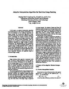
Fig. 1. The evolution process of the TRD model. It starts from an initial point 𝑢0 with energy functional 𝐸0 , goes to a new point 𝑢1 via a gradient descent step in the energy 𝐸0 , and then repeats this step with a new energy functional 𝐸1 until the end is reached.
(a) 2𝐷 𝑖𝑚𝑎𝑔𝑒.
(b) 1𝐷 𝑣𝑒𝑐𝑡𝑜𝑟𝑖𝑧𝑒𝑑 𝑖𝑚𝑎𝑔𝑒.
Fig. 2. Downsampling operator in upscaling factor 𝐿 = 2.
where 𝑘𝑡𝑖 are time varying convolution filters, 𝜙𝑡𝑖 are time varying influence functions1 (not restricted to be of a certain kind), and 𝜓(𝑢𝑡 , 𝑓 ) is the reaction term. Note that these parameters are trained from samples. In practice, the TRD model (5) can be trained for specific image restoration problem by exploiting application specific reaction terms 𝜓(𝑢). For classical image restoration problems, such as Gaussian denoising, image deblurring, image super resolution and image interpolation, we can set the reaction term to be the gradient of a data term, i.e., 𝜓(𝑢) = ∇𝑢 (𝑢). Eq. (5) can be interpreted as a gradient descent step at 𝑢𝑡−1 for the energy functional given by 𝐸 𝑡 (𝑢, 𝑓 ) =
𝑁𝑘 ∑
𝑡𝑖 (𝑢) + 𝑡 (𝑢, 𝑓 ) ,
parameters {𝑘𝑡𝑖 , 𝜌𝑡𝑖 } change with time 𝑡, Eq. (6) is a dynamic energy functional, which vary at each iteration 𝑡. The evolution process associated with Eq. (5) is illustrated in Fig. 1. From Fig. 1, one can see that the TRD model is to optimize a time-discrete PDE. It directly learns an optimal trajectory for a certain possibly unknown energy functional, the minimizer of which provides a good estimate of the demanded solution. Probably, such a functional cannot be modeled by a single energy, while the learned gradient descent steps provide good approximation to the local gradients of this unknown functional. 2.3. Image interpolation with the TRD framework In this paper, we exploit the TRD framework for the problem of image interpolation, coined as ITRD. According to the single image interpolation degradation model (1), the data term for single image interpolation problem discussed in this work is (𝑢, 𝑓 ) = 𝜆2 ‖𝐷𝑢 − 𝑓 ‖22 , where 𝜆 is related to the strength of the data term, 𝐷 is the downsampling operator that downsamples the HR image by a factor of 𝐿 in each axis. Taking upscaling factor of 𝐿 = 2 as an example, the downsampling and upsampling procedures are shown in Fig. 2(a). In this paper, the HR
(6)
𝑖=1
∑ 𝑡 𝑡 where 𝑡𝑖 (𝑢) = 𝑁 𝑝=1 𝜌𝑖 ((𝑘𝑖 ∗ 𝑢)𝑝 ) are the regularizers, and the functions 𝑡 𝜌𝑖 are the so-called penalty functions in the FoE models [17]. Since the 1 In the context of image regularization, the influence function 𝜙 is the first-order 𝑖 derivative of the penalty function 𝜌𝑖 in Eq. (6), i.e., 𝜙𝑖 (⋅) = 𝜌′𝑖 (⋅)
260
P. Qiao et al.
Signal Processing: Image Communication 58 (2017) 258–269 ′ ′ i.e., 𝐾𝑖 𝑢 ⇔ 𝑘𝑖 ∗ 𝑢, and 𝐾̄ 𝑖 𝑢 ⇔ 𝑘̄ 𝑖 ∗ 𝑢. 𝛬𝑖 = 𝑑𝑖𝑎𝑔(𝜙𝑡+1 (𝑧1 ), … , 𝜙𝑡+1 (𝑧𝑝 )) 𝑖 𝑖 with 𝑧 = 𝑘𝑡+1 ∗ 𝑢 , 𝑝 is the number of pixels in image. 𝑡 𝑖 Combine (10) and (11), we can get the gradient of 𝓁(𝑢𝑇 , 𝑢𝑔𝑡 ) w.r.t. 𝑢𝑡 . To make the derivation clear, we mark the gradient of 𝓁(𝑢𝑇 , 𝑢𝑔𝑡 ) w.r.t. 𝑢𝑡 as
and LR image are represented in vector form, Therefore, the size of 𝑢 and 𝑓 are R𝑝 and R𝑝𝐿 , respectively, where 𝑝 and 𝑝𝐿 are the number of pixels in the HR and LR image respectively. The downsampling operator 𝐷 is constructed as follow. The 𝑗th row of operator 𝐷 contains preciously one non-zero element (whose value is one) located at the position of the 𝑗th red rectangle in Fig. 2(b). Therefore, the downsampling operator 𝐷 is a matrix whose size is R𝑝𝐿 ×𝑝 , according to Eq. (1). The upsampling operator is simply the transpose of the downsampling operator 𝐷, as 𝐷T . Given the construction of the downsampling and upsampling operator 𝐷, the corresponding reaction term for image interpolation is set to 𝜓(𝑢) = 𝜆𝐷T (𝐷𝑢 − 𝑓 ). Therefore, the diffusion model (5) for single image interpolation can be written as 𝑁𝑘 ⎧ ∑ ⎪𝑢𝑡 = 𝑢𝑡−1 − 𝑘̄ 𝑡𝑖 ∗ 𝜙𝑡𝑖 (𝑘𝑡𝑖 ∗ 𝑢𝑡−1 ) − 𝜆𝑡 𝐷T (𝐷𝑢 − 𝑓 ), 𝑡 = 1 ⋯ 𝑇 ⎨ 𝑖=1 ⎪𝑢 = 𝐼, ⎩ 0
𝜕𝓁(𝑢𝑇 , 𝑢𝑔𝑡 ) 𝜕𝑢𝑡
The gradients of 𝓁(𝑢𝑇 , 𝑢𝑔𝑡 ) w.r.t. parameters 𝛩𝑡 are listed as below. gradients of
(7)
𝜕𝓁(𝑢𝑇 , 𝑢𝑔𝑡 ) 𝜕𝜆𝑡
𝜕𝑢𝑡 , 𝜕𝛩𝑡
we arrive the
.
𝜕𝓁(𝑢𝑇 ,𝑢𝑔𝑡 ) 𝜕𝜆𝑡
. The derivative of 𝑢𝑡
(13)
= (𝐷T (𝐷𝑢𝑡−1 − 𝑓 ))T 𝑒.
(14)
𝜕𝓁(𝑢𝑇 ,𝑢𝑔𝑡 ) The gradient of 𝓁(𝑢𝑇 , 𝑢𝑔𝑡 ) w.r.t. 𝑘𝑡𝑖 , . The gradient of 𝑢𝑡 𝜕𝑘𝑡𝑖
𝜕𝑢𝑡 𝜕𝑘𝑡𝑖
w.r.t.
⋅
𝜕𝑢𝑠𝑡+1 𝜕𝑢𝑠𝑡
⋯
𝜕𝓁(𝑢𝑠𝑇 , 𝑢𝑠𝑔𝑡 ) 𝜕𝑢𝑠𝑇
( ⊤ ⊤ ) ⊤ = − 𝛯𝑖𝑛𝑣 𝑌 + 𝑈𝑡−1 𝛬𝑖 (𝐾̄ 𝑖𝑡 )⊤ ,
𝑘𝑖 ∗ 𝑢𝑡−1 ⇔ 𝑈𝑡−1 𝑘𝑖 . The matrix 𝑌 is defined in the same way, and 𝑦 is given as 𝑦 = 𝜙𝑡𝑖 (𝐾𝑖𝑡 𝑢𝑡−1 ). ⊤ is a linear operator which inverts the vectorized kernel 𝑘. In Matrix 𝛯𝑖𝑛𝑣 the case of a square kernel 𝑘, it is equivalent to the Matlab command
(8)
⊤ 𝛯𝑖𝑛𝑣 𝑘 ⟺ 𝑟𝑜𝑡90(𝑟𝑜𝑡90(𝑘)) .
Combining the gradient in (12) and (15), the gradient of as 𝜕𝓁(𝑢𝑇 , 𝑢𝑔𝑡 ) ( ⊤ ⊤ ) ⊤ = − 𝛯𝑖𝑛𝑣 𝑌 + 𝑈𝑡−1 𝛬𝑖 (𝐾̄ 𝑖𝑡 )⊤ 𝑒 . 𝜕𝑘𝑡𝑖
𝑘𝑡𝑖 =
𝑐𝑖𝑡 . || 𝑡 || ||𝑐𝑖 || || ||2
from (17),
𝜕𝑐𝑖𝑡
𝜕𝑘𝑡𝑖 𝜕𝑐𝑖𝑡
, which is computed
=
The gradient of 𝓁(𝑢𝑇 , 𝑢𝑔𝑡 ) w.r.t. 𝜙𝑡𝑖 ,
is given as
𝜕𝓁(𝑢𝑇 ,𝑢𝑔𝑡 ) 𝜕𝜙𝑡𝑖
. Following the work
in [20], the nonlinear functions 𝜙𝑖 are parameterized via radial basis function (RBFs), i.e., function 𝜙𝑖 is represented as a weighted linear combination of a set of RBFs as follows, | | 𝑀 |𝑥 − 𝜇𝑗 | ∑ | | ), 𝜙𝑖 (𝑥) = 𝛼𝑖𝑗 𝜑( (19) 𝛾 𝑗=1
𝑁
𝑘 ∑ 𝜕𝑢𝑡+1 T = (𝐼 − 𝜆𝑡+1 𝐷T 𝐷) − 𝐾𝑖𝑡+1 𝛬𝑖 (𝐾̄ 𝑖𝑡+1 )T , 𝜕𝑢𝑡 𝑖=1
(16)
⎛ 𝑐𝑖𝑡 (𝑐 𝑡 )⊤ ⎞ 1 ⎜ 𝐼− ⋅ 𝑖 ⎟ ⋅ ⊤ . (18) || 𝑡 || ⎜ || 𝑡 || || 𝑡 || ⎟ ||𝑐𝑖 || ⎝ ||𝑐𝑖 || ||𝑐𝑖 || ⎠ || ||2 || ||2 || ||2 Combining the results of (18) and (16), we can obtain the required 𝜕𝓁(𝑢𝑇 ,𝑢𝑔𝑡 ) gradient of . 𝜕𝑐 𝑡 𝜕𝑘𝑡𝑖
𝑖
𝜕𝑢𝑡+1 𝜕𝑢𝑡
is given
(17)
We need to additionally calculate the gradient of
(10)
Given diffusion equation (7), the gradient of
𝜕𝓁 𝜕𝑘𝑡𝑖
To get rid of the scaling problem of the filter 𝑘𝑖 , it is necessary to fix the scale of the filter. Following the common used setting that meaningful filters should be zero-mean with unit norm, the filter 𝑘𝑖 is constructed from the Discrete Cosine Transform (DCT) basis omitting the DC-component. Therefore, the filter 𝑘𝑖 is defined as
For the sake of brevity, we only consider the case of one training sample, omitting 𝑠. It is easy to extend the result derivation to full training samples. It is easy to check that, for L2 loss function, the gradient of 𝓁(𝑢𝑇 , 𝑢𝑔𝑡 ) w.r.t. 𝑢𝑇 is given as = 𝑢𝑇 − 𝑢𝑔𝑡 .
′
′
(9)
.
(15)
where matrix 𝛬𝑖 is a diagonal matrix given as 𝛬𝑖 = diag(𝜙𝑡𝑖 (𝑧1 ), … , 𝜙𝑡𝑖 (𝑧𝑝 )) with 𝑧 = 𝐾𝑖𝑡 𝑢𝑡−1 . Matrix 𝑈𝑡−1 and 𝑌 are constructed from the images 𝑢𝑡−1 and 𝑦 of 2D form, respectively. For example, 𝑈𝑡−1 is constructed in the way that its rows are vectorized local patch extracted from image 𝑢𝑡−1 for each pixel, such that
The loss function 𝓁(𝑢𝑠𝑇 , 𝑢𝑠𝑔𝑡 ) in (8) is usually set to the L2 loss function defined as 12 ‖𝑢𝑠𝑇 − 𝑢𝑠𝑔𝑡 ‖2 . In this work, we also investigate the SSIM loss 2 function as [24]. The optimization problem in (8) can be solved via gradient based algorithms, e.g., commonly used L-BFGS algorithm [25]. The gradients of the loss function 𝓁(𝑢𝑠𝑇 , 𝑢𝑠𝑔𝑡 ) w.r.t. 𝛩𝑡 are computed using the standard back-propagation technique widely used in the neural networks learning [26]. Therefore, the general rule to compute the required gradients is give as
𝜕𝑢𝑇
and
𝑘𝑡𝑖 is formulated as
⎧ ⎪min (𝛩) = 𝓁(𝑢𝑠𝑇 , 𝑢𝑠𝑔𝑡 ) ⎪ 𝛩 𝑠=1 ⎪ (𝑁 ) 𝑘 ∑ ⎨ ⎧ 𝑠 𝑘̄ 𝑡𝑖 ∗ 𝜙𝑡𝑖 (𝑘𝑡𝑖 ∗ 𝑢𝑠𝑡−1 ) + 𝜆𝑡 𝐷T (𝐷𝑢𝑠𝑡−1 − 𝑓 𝑠 ) , ⎪ ⎪𝑢𝑡 = 𝑢𝑠𝑡−1 − ⎪𝑠.𝑡. ⎨ 𝑖=1 ⎪ ⎪ 𝑠 𝑠 ⎩ ⎩𝑢0 = 𝐼 , 𝑡 = 1 ⋯ 𝑇 .
𝜕𝓁(𝑢𝑇 , 𝑢𝑔𝑡 )
𝜕𝑢𝑡
Then the derivative of 𝓁(𝑢𝑇 , 𝑢𝑔𝑡 ) w.r.t. 𝜆𝑡 is
𝑆 ∑
𝜕𝛩𝑡
𝜕𝓁(𝑢𝑇 ,𝑢𝑔𝑡 )
𝜕𝑢𝑡 = 𝐷T (𝐷𝑢𝑡−1 − 𝑓 ), 𝜕𝜆𝑡
Inspired by [20], the model parameters 𝛩 = {𝛩𝑡 }𝑇𝑡=1 in ITRD are trained in a supervised manner. Therefore, we firstly prepare the input/output pairs, and then exploit a loss minimization scheme to learn the model parameters 𝛩 = {𝛩𝑡 }𝑇𝑡=1 . The training dataset consists of 𝑆 training samples {𝑓 𝑠 , 𝑢𝑠𝑔𝑡 }𝑆𝑠=1 , where 𝑢𝑠𝑔𝑡 is the clean HR image, and 𝑓 𝑠 is the corresponding LR image generated by (1). The training task is formulated as the following optimization problem
=
𝜕𝛩𝑡
Then, combining
The derivative of 𝓁(𝑢𝑇 , 𝑢𝑔𝑡 ) w.r.t. 𝜆𝑡 , w.r.t. 𝜆𝑡 is formulated as
2.4. ITRD training
𝜕𝑢𝑠𝑡
𝜕𝑢𝑡 . 𝜕𝛩𝑡 𝜕𝓁(𝑢𝑇 ,𝑢𝑔𝑡 )
First, we give the
where the initial point 𝐼 of the diffusion process (7) is simply set as the bicubic interpolation of the LR image 𝑓 . The ITRD model parameters 𝛩𝑡 of stage 𝑡 include the parameters of (1) the reaction force weight 𝜆𝑡 , (2) linear filters 𝑘𝑡𝑖 and (3) influence functions 𝜙𝑡𝑖 , i.e., 𝛩𝑡 = {𝜆𝑡 , 𝜙𝑡𝑖 , 𝑘𝑡𝑖 }.
𝜕𝓁(𝑢𝑠𝑇 , 𝑢𝑠𝑔𝑡 ) 𝜕𝛩𝑡
(12)
= 𝑒.
(11)
where {𝐾𝑖 , 𝐾̄ 𝑖 } ∈ R𝑝×𝑝 are highly sparse matrices, implemented as 2D convolution of the image 𝑢 with the filter kernel 𝑘𝑖 and 𝑘̄ 𝑖 , respectively, 261
P. Qiao et al.
Signal Processing: Image Communication 58 (2017) 258–269
Fig. 3. Test images from left to right and top to down: Elk, Bears, Boat, Butterfly, Koala, Cameraman, Texture, Fence, Flowers, Foreman, Girl, House, Leaves, Lena, Parrot, Parthenon, Starfish, and Stream. Table 1 Influence of inference stage 𝑇 . Average PSNR (dB), SSIM and inference time (s) on test images.
where 𝜑(⋅) here is Gaussian RBFs with equidistant centers 𝜇𝑗 and unified scaling 𝛾. 𝑀 is the number of Gaussian RBF. The Gaussian radial basis is defined as ( ) ( ) |𝑥 − 𝜇| (𝑥 − 𝜇)2 𝜑 = exp − 2 𝛾 2𝛾 For every pixel in 𝑧 = 𝑘𝑡𝑖 ∗ 𝑢𝑡−1 , Eq. (19) can be re-written in matrix form, 𝐺𝛼𝑖𝑡 = 𝜙𝑡𝑖 ,
𝜕𝑢𝑡
= −𝐺⊤ (𝐾̄ 𝑖𝑡 )⊤ ,
(21)
Therefore, The gradient of 𝓁(𝑢𝑇 , 𝑢𝑔𝑡 ) w.r.t. 𝛼𝑖𝑡 is given as 𝜕𝓁(𝑢𝑇 , 𝑢𝑔𝑡 ) 𝜕𝛼𝑖𝑡
= −𝐺⊤ (𝐾̄ 𝑖𝑡 )⊤ 𝑒 .
2
5
8
PSNR SSIM time
26.17 0.7819 0.59
26.27 0.7850 1.43
26.30 0.7863 2.00
Table 2 Influence of filter size 𝑚 × 𝑚. Average PSNR (dB), SSIM and inference time (s) on test images.
(20)
|𝑧 −𝜇 | where 𝐺𝑟𝑐 = 𝜑( 𝑟 𝛾 𝑐 ), 𝐺 ∈ 𝑝×𝑀 , 𝑟 = 1, … , 𝑝 and 𝑐 = 1, … , 𝑀. The gradient of 𝑢𝑡 w.r.t. 𝛼𝑖𝑡 is formulated as 𝜕𝛼𝑖𝑡
𝑇
𝑚×𝑚
3 × 3
5 × 5
7 × 7
PSNR SSIM time
25.80 0.7706 0.80
26.20 0.7832 1.25
26.27 0.7850 1.43
space, (ii) interpolate the luminance channel (i.e., Y) using the proposed algorithm and interpolate the chromatic channels (i.e., Cb and Cr) using the bi-cubic method, and (iii) convert the interpolated channels back to RGB color space. We evaluated the interpolation performance using the PSNR as [8] and SSIM as [27]. Only luminance channel is used in the evaluation. The comparison single image interpolation methods we used were downloaded from the author’s homepage or acquired via e-mail.
(22)
3. Experimental results 3.1. Training of ITRD models
3.2. Influence of inference stage
Concerning the model capacity, the stages of inference 𝑇 is set to 2, 5 and 8; the filter size 𝑚 × 𝑚 is set to 3 × 3, 5 × 5 and 7 × 7; the loss function in (8) is set to L2 and SSIM loss function. We trained the ITRD model for three upsampling factors: 𝐿 = 2, 3 and 4. The resulting models are denoted as ITRD𝑇𝑚×𝑚, 𝐿 . We used 400 training images of size 180 × 180 as those in [20]. The 400 images consist of the HR images {𝑢𝑠𝑔𝑡 }𝑆𝑠=1 . The corresponding LR images are {𝑓 𝑠 }𝑆𝑠=1 . The LR image is generated by 𝑓 𝑠 = 𝐷𝑢𝑠𝑔𝑡 , where 𝐷 is the downsampling operator parameterized by scaling factor 𝐿. We minimized the optimization problem (8) to learn the parameters of the ITRD modes with gradient-base L-BFGS [25]. The gradients of loss function w.r.t. the parameters can be derived from (9)–(22). We jointly trained the parameters of all stages. Computing the gradients of one stage for 400 images of size 180 × 180 takes about 211𝑠 on a server with CPUs: Intel(R) Xeon E5-2650 @ 2.00 GHz (eight cores). We run 250 L-BFGS iterations for optimization. Therefore, the total training time, e.g., for ITRD57×7, 3 model is 5 × (250 × 221)∕3600 = 76.7 h. In order to perform a fair comparison to previous works, i.e., SAI [6], CG [7], NAMR [8] and ANSM [9] algorithm, we used the images exploited in [9], namely Elk, Bears, Boat, Butterfly, Koala, Cameraman, Texture, Fence, Flowers, Foreman, Girl, House, Leaves, Lena, Parrot, Parthenon, Starfish, and Stream (see Fig. 3). Note that the training images and test images do not overlap. All the tests in this section are generated by decimating the input HR image by factor of 𝐿 in each axis. We tested the proposed algorithm for three scaling factors, 𝐿 = 2, 𝐿 = 3 and 𝐿 = 4. We followed the routine in [9] for processing color images: (i) convert the LR image 𝑓 𝑠 from RGB to YCbCr color
To investigate the influence of the inference stage, we fix the filter size 𝑚 × 𝑚 = 7 × 7, downsampling factor 𝐿 = 3, L2 loss function, and set inference stage 𝑇 to 2, 5, and 8. As described in Table 1, with the increase of inference stage 𝑇 , the interpolation performance is increasing. Note that the inference time increases linearly w.r.t. 𝑇 , while the performance increases marginally. To balance the inference efficiency and interpolation performance, inference stage 𝑇 = 5 is preferred. Unless explicitly stated, we set 𝑇 = 5 in the following experiment. 3.3. Influence of filter size To investigate the influence of the filter size, we fix the downsampling factor 𝐿 = 3, L2 loss function, and set 𝑚 × 𝑚 to 3 × 3, 5 × 5 and 7 × 7. As described in Table 2, with the increase of filter size 𝑚 × 𝑚, the interpolation performance is increasing. Note that the inference time increases a little, while the interpolation performance increases significantly. To balance the inference efficiency and interpolation performance, filter size 𝑚 × 𝑚 = 7 × 7 is preferred. The learned filters for ITRD57×7, 3 in the first and last stage are shown in Fig. 4. Unless explicitly stated, we set 𝑚 × 𝑚 = 7 × 7 in the following experiment. 3.4. Influence of loss function In [24,28], the loss function for discriminative training image restoration models is SSIM instead of L2. The trained models with SSIM 262
P. Qiao et al.
Signal Processing: Image Communication 58 (2017) 258–269
(a) 𝑠𝑡𝑎𝑔𝑒 = 1.
(a) L2-loss.
(b) SSIM-loss.
(c) L2-loss.
(d) SSIM-loss.
(e) L2-loss.
(f) SSIM-loss.
(g) L2-loss.
(h) SSIM-loss.
(b) 𝑠𝑡𝑎𝑔𝑒 = 5.
Fig. 4. The learned filters for ITRD57×7, 3 in the first and last stage. Table 3 Influence of loss function. Average PSNR (dB) and SSIM on test images. Inference
Training 𝐿=2
PSNR SSIM
𝐿=3
𝐿=4
L2
SSIM
L2
SSIM
L2
SSIM
30.05 0.8860
29.87 0.8918
26.27 0.7850
26.08 0.8005
24.35 0.7088
24.07 0.7291
Table 4 The runtime (s) comparison. Take 𝐿 = 2 as an example. Resolution
Bicubic
SAI [6]
CG [7]
NARM [8]
ANSM [9]
Ours
2562 5122 6402
0.03 0.05 0.05
0.44 1.85 2.89
0.45 2.06 3.34
100 485 994
2663 18518 22141
0.82 3.06 3.28
loss function may provide visually more plausible results. Inspired by these works, we also investigate the influence of loss function. We trained our ITRD models using L2 and SSIM loss function respectively. As described in 3, the model trained using L2 loss, coined as ITRDL2 , achieves higher PSNR compared with model trained using SSIM loss, coined as ITRDSSIM . By contrast, ITRDSSIM achieves higher SSIM compared with ITRDL2 . While the interpolated image produced by ITRDSSIM is visually plausible and with high contrast, the interpolated image may contain more artifacts, which is indicated by the lower PSNRs than that of ITRDL2 , as shown in Fig. 5. It is preferred that upsampling the LR image to recover correct details, though ITRDSSIM provides quite high image interpolation performance in terms of SSIM, as shown in Figs. 7(d)–7(f).
Fig. 5. The influence of loss function. Image Fence in upscaling factor of 𝐿 = 3. (a) interpolated image by ITRDL2 , (b) interpolated image by ITRDSSIM , (c) error map w.r.t. original HR image by ITRDL2 , (d) error map w.r.t. original HR image by ITRDSSIM . The second row are the zoom-in images in the red rectangle area of the first row respectively.
complexity, we can conclude that our ITRD model runs slower than SAI, as fast as CG, and faster than NARM and ANSM. We make the runtime comparison to other image interpolation algorithms based on strictly enforced single-thread CPU computation for the sake of fair comparison. The evaluation platform is Intel(R) CPU i5-4460 @ 3.20 GHz, and 8GB RAM. All comparison methods are implemented and tested in Matlab 2012b, except SAI which is in binary executable form. The image size impacts the runtime of all comparison methods regardless of upscaling factor 𝐿. For SAI and CG in 𝐿 = 3, though the input LR image is interpolated twice, the overall runtime is still short. For NARM and ANSM in 𝐿 = 4, though the input LR image is interpolated twice as well, the overall runtime does not increase significantly. Due to the image size of the first interpolation is small, the first interpolation is quite fast. Taking these into consideration, we show runtime comparison for 𝐿 = 2. Shown in Table 4, our model ITRD runs slower than SAI, on par with CG, and significantly faster than NARM and ANSM. We plot the time-interpolation performance in semilog coordinates. Illustrated in Fig. 6, we can conclude that our ITRD model runs about 2 to 4 orders of magnitude fast, and achieves promising single image interpolation quality as the state-of-the-art methods, e.g., NARM and ANSM. Compared with efficient approaches, our ITRD model offers significantly better image interpolation performance while runs as fast as
3.5. Runtime The computational complexity of ANSM is 𝑂(𝑇 ⋅ 𝑛3 ⋅ 𝑝),2 where 𝑇 is the number of iterations, 𝑛 is the patch size, 𝑝 is the number of pixels in the test image. The computational complexity of NARM is 𝑂(𝑇 ⋅ 𝑛 ⋅ 𝑝2 ) following the computational complexity analysis in [9]. The computational complexity of SAI is 𝑂(𝑎 ⋅ 𝑝), where 𝑎 is a small constant.3 The computational complexity of CG is 𝑂(𝑇 ⋅ 𝑎 ⋅ 𝑝).4 The computational complexity of ITRD is 𝑂(𝑇 ⋅ 𝑛 ⋅ 𝑝). From the comparison of computational 2 The computational complexity of ANSM is 𝑂(𝑇 ⋅ 𝑛3 ⋅ (𝑛2.5 + 𝑝)), where 𝑛2.5 ≪ 𝑝, and thus it can be approximated as 𝑂(𝑇 ⋅ 𝑛3 ⋅ 𝑝). 3 As described in [6], SAI is merely consist of three closed solution of least-square problem. Each solution runs in a constant time. Hence, we denote the maximal constant time of the three least-square solution as 𝑎. 4 As described in [7], CG is a diffusion-like approach, which runs a few diffusion steps until convergence.
263
P. Qiao et al.
Signal Processing: Image Communication 58 (2017) 258–269
(a) 𝐿 = 2.
(b) 𝐿 = 3.
(c) 𝐿 = 4.
(d) 𝐿 = 2.
(e) 𝐿 = 3.
(f) 𝐿 = 4.
Fig. 6. Speed vs. PSNR/SSIM over 18 tested images for the tested methods in (a, d) 𝐿 = 2, (b, e) 𝐿 = 3 and (c, f) 𝐿 = 4 scenarios. The first row is speed vs. PSNR. The second row is speed vs. SSIM. Note we plot the comparison in semilog coordinates.
(a) 𝐿 = 2.
(b) 𝐿 = 3.
(c) 𝐿 = 4.
(d) 𝐿 = 2.
(e) 𝐿 = 3.
(f) 𝐿 = 4.
Fig. 7. Scatter plot of the PSNRs/SSIMs over 18 test images produced by our ITRD model, SAI, CG, NARM, ANSM in 𝐿 = 2, 𝐿 = 3 and 𝐿 = 4 scenarios. The first row shows PSNR comparison, the second row shows SSIM comparison. Points above the diagonal line mean a better performance than our model, whereas points below this line indicate inferior results.
SAI and CG. On one hand, our ITRD model takes a few stages diffusion, at each diffusion stage merely contains the convolution operation with a few linear filters. On the other hand, the promising single image
interpolation quality benefits from the trained linear filters and the trained influence functions, which are time-varying. Our ITRD model can run even faster via GPU implementation of convolution. 264
P. Qiao et al.
Signal Processing: Image Communication 58 (2017) 258–269
Table 5 The interpolation results (PSNR/SSIM) for 𝐿 = 2. Image
Bicubic
SAI [6]
CG [7]
NARM [8]
ANSM [9]
0urs L2 loss
Ours SSIM loss
House Foreman Partheon Cameraman Fence Girl Parrot Boat Flowers Stream Elk Lena Leaves Butterfly Starfish Texture Bears Koala
32.16 / 0.8772 35.58 / 0.9491 27.08 / 0.8043 25.35 / 0.8639 24.52 / 0.7775 33.83 / 0.8533 26.17 / 0.8847 29.23 / 0.8407 28.09 / 0.8151 25.82 / 0.7975 31.58 / 0.9255 33.92 / 0.9140 26.85 / 0.9365 27.68 / 0.9242 30.22 / 0.9168 20.53 / 0.8483 28.50 / 0.8800 33.24 / 0.9140
32.84 / 0.8778 37.68 / 0.9576 27.10 / 0.8014 25.88 / 0.8709 23.77 / 0.7704 34.13 / 0.8588 27.01 / 0.8948 29.69 / 0.8477 28.84 / 0.8343 25.92 / 0.7984 33.06 / 0.9353 34.68 / 0.9184 28.72 / 0.9575 29.17 / 0.9468 30.77 / 0.9208 21.48 / 0.8768 28.53 / 0.8803 33.75 / 0.9163
32.81 / 0.8805 37.40 / 0.9555 27.10 / 0.8027 25.86 / 0.8694 24.59 / 0.7823 33.97 / 0.8547 26.60 / 0.8901 29.51 / 0.8430 28.54 / 0.8250 25.68 / 0.7924 32.76 / 0.9323 34.44 / 0.9162 28.12 / 0.9511 28.86 / 0.9426 30.43 / 0.9169 21.40 / 0.8758 28.18 / 0.8754 33.54 / 0.9130
33.44 / 0.8843 38.68 / 0.9581 27.31 / 0.8074 25.91 / 0.8754 24.71 / 0.7916 34.44 / 0.8649 26.83 / 0.8935 29.80 / 0.8567 28.81 / 0.8362 25.84 / 0.8007 33.21 / 0.9355 35.02 / 0.9234 29.69 / 0.9663 30.29 / 0.9556 31.72 / 0.9298 21.43 / 0.8778 28.31 / 0.8802 33.81 / 0.9135
34.34 / 0.8898 38.37 / 0.9589 27.33 / 0.8034 26.49 / 0.8791 24.77 / 0.7923 34.24 / 0.8618 27.04 / 0.8939 30.12 / 0.8571 28.88 / 0.8366 26.02 / 0.7998 33.70 / 0.9392 34.79 / 0.9212 29.08 / 0.9609 29.75 / 0.9522 31.05 / 0.9240 22.06 / 0.8937 28.64 / 0.8800 33.83 / 0.9169
34.30 / 0.8971 38.17 / 0.9572 27.92 / 0.8242 26.23 / 0.8786 24.56 / 0.7867 34.35 / 0.8622 26.94 / 0.8920 30.08 / 0.8548 29.12 / 0.8369 26.04 / 0.7965 33.66 / 0.9359 34.62 / 0.9196 29.28 / 0.9593 30.04 / 0.9495 31.40 / 0.9249 21.67 / 0.8828 28.79 / 0.8793 33.82 / 0.9111
34.01 / 0.8975 37.86 / 0.9590 27.58 / 0.8307 26.08 / 0.8839 24.48 / 0.8002 34.11 / 0.8643 26.99 / 0.8978 29.83 / 0.8578 28.84 / 0.8428 25.79 / 0.8100 33.40 / 0.9401 34.57 / 0.9230 29.25 / 0.9649 29.85 / 0.9533 31.40 / 0.9326 21.52 / 0.8876 28.52 / 0.8885 33.65 / 0.9186
Average
28.91 / 0.8735
29.61 / 0.8814
29.43 / 0.8788
29.96 / 0.8862
30.03 / 0.8867
30.05 / 0.8860
29.87 / 0.8918
(a) Input.
(e) Input.
(i) ANSM.
(m) ANSM.
(b) Original.
(f) Original.
(j) NARM.
(n) NARM.
(c) Bicubic.
(g) Bicubic.
(k) SAI.
(o) SAI.
(d) Ours. (a) Input.
(b) Original.
(c) bicubic.
(d) Ours.
(e) Input.
(f) Original.
(g) bicubic.
(h) Ours.
(h) Ours.
(l) CG.
(i) ANSM.
(j) NARM.
(k) SAI.
(l) CG.
(m) ANSM.
(n) NARM.
(o) SAI.
(p) CG.
(p) CG.
Fig. 8. Visual comparison of interpolated image in 𝐿 = 2 scenario for parthenon. From left to right and top to bottom, images are produced by the decimate downsampling, original, bicubic, our ITRD model, ANSM, NARM, SAI and CG, respectively. The cropped images are put below the corresponding produced images.
Fig. 9. Visual comparison of interpolated image in 𝐿 = 2 scenario for fence. From left to right and top to bottom, images are produced by the decimate downsampling, original, bicubic, our ITRD model, ANSM, NARM, SAI and CG, respectively. The cropped images are put below the corresponding produced images.
3.6. Up-scaling by a factor of 2 For single image interpolation by factor of 𝐿 = 2, our ITRD57×7, 2 is competitive compared with ANSM and NARM, and surpasses SAI, CG, and bicubic, as shown in Fig. 7(a). From Table 5, we can see that our ITRD57×7, 2 surpasses bicubic, SAI, CG, and NARM by 1.1dB, 0.4dB, 0.6dB, and 0.1dB in average respectively.5 Note that our ITRD57×7, 2 surpasses both NARM and ANSM in four test images, i.e., Bears, Flowers,
Pantheon and Stream. Taking image Pantheon as an example, our ITRD57×7, 2 produces vertical structures in the pillars of the Pantheon, whereas NARM and ANSM trend to keep the bi-cubic slash artifacts unchanged, as illuminated in Fig. 8. In image Fence and Foreman, our model do not work well in the recovering of large line structures, as shown in Fig. 9. This is not surprising that our model exploits merely
5
Note that the implementation of the NARM algorithm from the authors’ homepage failed to exactly reproduce the interpolation results presented in [8], even with the authors’ guide.
local information, whereas NAMR and ANSM benefit from the non-local redundancy. 265
P. Qiao et al.
Signal Processing: Image Communication 58 (2017) 258–269
Table 6 The interpolation results (PSNR/SSIM) for 𝐿 = 3. Image
Bicubic
SAI [6]
CG [7]
NARM [8]
ANSM [9]
ours L2 loss
Ours SSIM loss
House Foreman Partheon Cameraman Fence Girl Parrot Boat Flowers Stream Elk Lena Leaves Butterfly Starfish Texture Bears Koala
28.66 / 0.8190 32.08 / 0.9079 24.28 / 0.6789 22.35 / 0.7686 20.64 / 0.5941 31.45 / 0.7771 22.81 / 0.8011 26.00 / 0.7453 25.82 / 0.7233 23.11 / 0.6457 27.95 / 0.8514 30.14 / 0.8550 21.85 / 0.8166 23.47 / 0.8236 26.16 / 0.8135 16.38 / 0.6432 25.43 / 0.7681 29.59 / 0.8171
29.06 / 0.8252 33.58 / 0.9237 24.51 / 0.6821 22.73 / 0.7797 20.23 / 0.5870 31.78 / 0.7831 23.24 / 0.8149 26.35 / 0.7513 26.26 / 0.7378 23.18 / 0.6399 28.62 / 0.8628 30.88 / 0.8650 22.80 / 0.8594 24.61 / 0.8748 26.31 / 0.8139 16.83 / 0.6712 25.54 / 0.7676 30.00 / 0.8213
28.97 / 0.8250 33.39 / 0.9205 24.32 / 0.6776 22.64 / 0.7778 20.62 / 0.5902 31.68 / 0.7805 23.23 / 0.8141 26.15 / 0.7480 26.08 / 0.7321 23.00 / 0.6351 28.62 / 0.8602 30.68 / 0.8627 22.51 / 0.8494 24.42 / 0.8669 25.96 / 0.8052 16.93 / 0.6891 25.34 / 0.7648 29.86 / 0.8184
29.72 / 0.8350 34.44 / 0.9170 24.70 / 0.6903 22.65 / 0.7840 20.65 / 0.6025 31.83 / 0.7806 23.32 / 0.8127 26.53 / 0.7632 26.47 / 0.7431 23.20 / 0.6437 28.90 / 0.8605 31.18 / 0.8683 23.35 / 0.8797 25.47 / 0.8960 26.78 / 0.8270 16.62 / 0.6689 25.37 / 0.7652 30.08 / 0.8119
30.23 / 0.8443 35.02 / 0.9324 24.77 / 0.6928 23.11 / 0.7925 20.61 / 0.6088 32.00 / 0.7911 23.76 / 0.8231 26.78 / 0.7648 26.46 / 0.7437 23.40 / 0.6472 29.19 / 0.8699 31.14 / 0.8697 23.34 / 0.8759 25.42 / 0.8934 26.70 / 0.8258 17.31 / 0.7053 25.75 / 0.7716 30.31 / 0.8278
29.63 / 0.8405 34.09 / 0.9242 24.94 / 0.6944 23.18 / 0.7913 20.92 / 0.6113 32.03 / 0.7875 23.48 / 0.8111 26.56 / 0.7557 26.58 / 0.7406 23.42 / 0.6318 29.48 / 0.8668 30.85 / 0.8630 22.87 / 0.8556 24.95 / 0.8785 26.54 / 0.8120 17.29 / 0.6876 25.98 / 0.7662 30.13 / 0.8122
29.52 / 0.8466 34.10 / 0.9303 24.48 / 0.7085 22.83 / 0.8018 20.53 / 0.6303 31.89 / 0.7939 23.38 / 0.8249 26.43 / 0.7689 26.35 / 0.7561 22.99 / 0.6615 29.19 / 0.8780 30.76 / 0.8719 23.05 / 0.8823 25.09 / 0.8936 26.56 / 0.8369 16.80 / 0.7056 25.45 / 0.7872 30.01 / 0.8307
Average
25.45 / 0.7694
25.92 / 0.7811
25.80 / 0.7788
26.18 / 0.7861
26.40 / 0.7933
26.27 / 0.7850
26.08 / 0.8005
(a) Input.
(b) Original.
(c) Bicubic.
(d) Ours.
(e) Input.
(f) Original.
(g) Bicubic.
(h) Ours.
(i) ANSM
(m) ANSM.
(j) NARM.
(n) NARM.
(k) SAI.
(o) SAI.
(a) Input.
(b) Original.
(c) Bicubic.
(d) Ours.
(e) Input.
(f) Original.
(g) Bicubic.
(h) Ours.
(l) CG. (i) ANSM.
(j) NARM.
(k) SAI.
(l) CG.
(m) ANSM.
(n) NARM.
(o) SAI.
(p) CG.
(p) CG.
Fig. 10. Visual comparison of interpolated image in 𝐿 = 3 scenario for elk. From left to right and top to bottom, images are produced by the decimate downsampling, original, bicubic, our ITRD model, ANSM, NARM, SAI and CG, respectively. The cropped images are put below the corresponding produced images.
Fig. 11. Visual comparison of interpolated image in 𝐿 = 3 scenario for foreman. From left to right and top to bottom, images are produced by the decimate downsampling, original, bicubic, our ITRD model, ANSM, NARM, SAI and CG, respectively. The cropped images are put below the corresponding produced images.
3.7. Up-scaling by a factor of 3 LR images twice by a factor of 𝐿 = 2, (ii) and then reduced the results by a factor of 34 using the bicubic interpolation. The implementation of CG also does not support upscaling of factors 𝐿 = 3, we followed the same way as that for SAI. Our ITRD57×7, 3 is competitive compared with ANSM and NARM, and surpasses SAI, CG, and bicubic, as shown in Fig. 7(b). According
For single image interpolation by factor of 𝐿 = 3, since the available implementations for SAI do not support upscaling of factors other than 2, we followed the same way described in [9],6 : (i) first interpolated the 6 In [6] the author suggest that for 𝐿 ≠ 2𝑧 , 𝑧 ∈ Z+ , one can upsample the LR image using SAI with upscale factor of 𝑠, 𝑠 = 2𝑧 , 𝑠 < 𝐿, 𝑧 ∈ Z+ , then upsample the SAI output to 𝐿 using bicubic upsampling method with 𝑆, 𝑠𝑆 = 𝐿, 𝑠 = 2𝑧 , 𝑠 < 𝐿, 𝑧 ∈ Z+ . Following above upsampling scheme, the output interpolated image is worse than that produced
using scheme in [9]. Therefore, we choose latter to interpolate LR image when using SAI and CG. 266
P. Qiao et al.
Signal Processing: Image Communication 58 (2017) 258–269
Table 7 The interpolation results (PSNR/SSIM) for 𝐿 = 4 Image
Bicubic
SAI [6]
CG [7]
NARM [8]
ANSM [9]
Ours L2 loss
Ours SSIM loss
House Foreman Partheon Cameraman Fence Girl Parrot Boat Flowers Stream Elk Lena Leaves Butterfly Starfish Texture Bears Koala
26.58 / 0.7682 30.02 / 0.8730 23.09 / 0.6115 21.11 / 0.7131 18.99 / 0.4801 29.91 / 0.7299 20.58 / 0.7290 24.17 / 0.6715 24.36 / 0.6618 21.71 / 0.5430 26.31 / 0.8089 27.94 / 0.8085 19.27 / 0.7035 21.31 / 0.7416 24.15 / 0.7346 14.22 / 0.4693 24.32 / 0.7054 27.70 / 0.7410
27.16 / 0.7854 31.06 / 0.8922 23.36 / 0.6198 21.63 / 0.7285 18.68 / 0.4812 30.35 / 0.7402 21.12 / 0.7532 24.61 / 0.6831 24.71 / 0.6757 21.83 / 0.5399 26.96 / 0.8214 28.80 / 0.8262 20.10 / 0.7655 22.13 / 0.8043 24.31 / 0.7357 14.50 / 0.4946 24.34 / 0.7071 28.10 / 0.7494
26.94 / 0.7789 31.25 / 0.8918 23.16 / 0.6128 21.37 / 0.7227 19.02 / 0.4859 30.24 / 0.7364 21.00 / 0.7500 24.42 / 0.6785 24.47 / 0.6678 21.65 / 0.5371 26.77 / 0.8149 28.62 / 0.8239 19.85 / 0.7515 21.95 / 0.7939 23.96 / 0.7205 14.47 / 0.5120 24.18 / 0.7023 28.03 / 0.7478
27.42 / 0.7948 31.73 / 0.8986 23.30 / 0.6243 21.13 / 0.7266 18.81 / 0.4832 30.57 / 0.7444 20.68 / 0.7486 24.40 / 0.6887 24.58 / 0.6757 21.58 / 0.5410 26.92 / 0.8219 28.78 / 0.8311 19.60 / 0.7618 22.28 / 0.8133 24.59 / 0.7549 13.98 / 0.4694 24.07 / 0.7069 28.11 / 0.7493
27.49 / 0.7945 32.45 / 0.9042 23.56 / 0.6280 21.75 / 0.7333 18.49 / 0.4734 30.46 / 0.7454 21.21 / 0.7465 24.93 / 0.6945 24.83 / 0.6761 21.97 / 0.5409 27.10 / 0.8261 28.86 / 0.8282 20.54 / 0.7838 22.30 / 0.8138 24.54 / 0.7392 14.75 / 0.5166 24.74 / 0.7106 28.44 / 0.7585
27.24 / 0.7921 31.46 / 0.8875 23.70 / 0.6236 21.97 / 0.7373 19.64 / 0.5088 30.56 / 0.7393 21.22 / 0.7402 24.80 / 0.6800 24.94 / 0.6677 22.20 / 0.5283 27.61 / 0.8284 28.58 / 0.8138 20.09 / 0.7588 21.95 / 0.7968 24.29 / 0.7179 15.00 / 0.4993 24.98 / 0.7007 28.17 / 0.7375
27.29 / 0.8048 31.53 / 0.8981 23.16 / 0.6388 21.57 / 0.7534 18.92 / 0.5240 30.36 / 0.7472 20.97 / 0.7582 24.45 / 0.6983 24.63 / 0.6911 21.61 / 0.5620 27.14 / 0.8384 28.50 / 0.8284 20.06 / 0.7929 22.19 / 0.8243 24.24 / 0.7555 14.35 / 0.5252 24.29 / 0.7230 28.00 / 0.7594
Average
23.65 / 0.6941
24.10 / 0.7113
23.96 / 0.7071
24.03 / 0.7130
24.36 / 0.7174
24.35 / 0.7088
24.07 / 0.7291
(a) NARM
(d) NARM.
(b) Ours.
(e) Ours.
(a) Input.
(b) Original.
(c) Bicubic.
(d) Ours.
(e) Input.
(f) Original.
(g) Bicubic.
(h) Ours.
(c) ANSM.
(f) ANSM.
Fig. 12. Visual comparison of interpolated image for fence. First row is for 𝐿 = 2, and second row is for 𝐿 = 3. From left to right, the images are from NARM, out ITRD model and ANSM.
to Table 6, our ITRD57×7, 3 surpass bicubic, SAI, CG, and NARM by 0.8dB, 0.3dB, 0.5dB, and 0.1dB in average respectively. Our ITRD57×7, 3 outperforms both ANSM and NARM in eight test images, i.e., Bears, Cameraman, Elk, Fence, Flowers, Girl, Pantheon and Stream. In image Elk, our ITRD57×7, 3 recovers the horn of the elk more preciously, as shown in Fig. 10. In image Foreman, our ITRD57×7, 3 encounters the same problems as that in 𝐿 = 2, as shown in Fig. 11. It is interesting that in image Fence, our ITRD57×7, 3 produces higher PSNR compared with those of ANSM and NARM. One notable detail, as illuminated in Fig. 12, our ITRD57×7, 3 recovers more structures in the eaves than ANSM and NARM. ANSM still finds non-local similar patches from the bicubic interpolation image in which the structures in the eaves are damaged, as shown in the third column of Fig. 12. On the contrary, our model recovers more details from the degraded images, as shown in the second column of Fig. 12. We can conclude that our ITRD model has amazing inferring ability to recover details, which is crucial for single image interpolation.
(i) ANSM.
(j) NARM.
(k) SAI.
(l) CG.
(m) ANSM.
(n) NARM.
(o) SAI.
(p) CG.
Fig. 13. Visual comparison of interpolated image in 𝐿 = 4 scenario for parrot. From left to right and top to bottom, images are produced by the decimate downsampling, original, bicubic, our ITRD model, ANSM, NARM, SAI and CG, respectively. The cropped images are put below the corresponding produced images.
used the parameter setting for 𝐿 = 2, and interpolated the LR images twice by a factor of 𝐿 = 2. Our ITRD57×7, 4 is competitive compared with ANSM, and surpasses NARM, SAI, CG, and bicubic, as shown in Fig. 7(c). According to Table 7, our ITRD57×7, 4 surpasses bicubic, SAI, CG, and NARM by 0.7dB, 0.25dB, 0.39dB, and 0.32dB in average respectively. Our ITRD57×7, 4 outperforms both ANSM and NARM in nine test images, i.e., Pantheon, Cameraman, Fence, Parrot, Flowers, Stream, Elk, Texture, Bears. In image Parrot, our ITRD57×7, 4 recovers the eye of parrot more preciously, as shown
3.8. Up-scaling by a factor of 4 For single image interpolation by factor of 𝐿 = 4, since NARM and ANSM do not provide parameter settings for this upscaling factor, we 267
P. Qiao et al.
(a) Input.
(e) Input.
(i) ANSM.
Signal Processing: Image Communication 58 (2017) 258–269
(b) Original.
(f) Original.
(c) Bicubic.
(g) Bicubic.
(j) NARM.
(k) SAI.
(d) Ours.
(a) Original.
(b) Bicubic.
(c) SRCNN.
(d) Ours.
(h) Ours.
(l) CG.
Fig. 15. Visual comparison of interpolated image in 𝐿 = 3 scenario for house. (m) ANSM.
(n) NARM.
(o) SAI.
(p) CG.
Fig. 14. Visual comparison of interpolated image in 𝐿 = 4 scenario for cameraman. From left to right and top to bottom, images are produced by the decimate downsampling, original, bicubic, our ITRD model, ANSM, NARM, SAI and CG, respectively. The cropped images are put below the corresponding produced images.
in Fig. 13. In image Cameraman, our ITRD57×7, 4 recovers camera more preciously, as shown in Fig. 14. (a) Original.
(b) Bicubic.
(c) SRCNN.
(d) Ours.
3.9. Comparison with CNN-based model In this work, we resort to a recently developed PDE-based image restoration framework — TRD. We prefer TRD due to its effectiveness and brevity, and more importantly, it has a clear picture from the aspect of energy minimization. To be specific, the resulting multistage network is derived from unrolling an optimization process. As a consequence, every single parameter in this multi-stage network has a clear interpretation why it should like this. Herein, we would like to clarify the difference between the TRD network and conventional CNN based image restoration models, such as SRCNN [29], or more recent VDSR model [30]. There are three important distinguishing characteristics: (1) TRD has a very unique architecture. Each convolution + nonlinearity operation is followed by a convolution operation which is rotated version of the previous convolution. On the contrary, convention CNN models do not contain such a convolution layer. The architecture of TRD is derived from energy minimization process. (2) TRD has adjustable nonlinearities. Note that the nonlinear functions in the TRD network is trainable. However, conventional CNN models make use of a fixed one, such as ReLU. (3) TRD has a clear explainability due to its essence from certain energy minimization process as mentioned above. However, at present, a convincing interpretation for conventional CNN models why it works or why it fails is still missing. Even though the TRD network can be treated as a convolution network, we do not want to categorize it as a conventional CNN method because of the above differentiae.
Fig. 16. Visual comparison of interpolated image in 𝐿 = 3 scenario for Elk.
For the task of image interpolation, we do have many choices to extend those image up-scaling algorithms developed for general image super-resolution problems, such as SRCNN, ANR and VDSR algorithm to this problem with proper re-training. And we do believe that these variants can work well for image interpolation. However, this is beyond the scope of our paper. Moreover, in our paper, we have already made intensive comparison to those recent algorithms NARM [8] and ANSM [9], which are especially developed for the task of image interpolation. As described above, image interpolation problem (1) is a special case of general image super-resolution problem (2). Given that there is no 268
P. Qiao et al.
Signal Processing: Image Communication 58 (2017) 258–269
Table 8 The interpolation results (PSNR/SSIM) for 𝐿 = 3. Image
Bicubic
NARM [8]
ANSM [9]
Ours L2 loss
ours SSIM loss
SRCNN [29]
House Foreman Partheon Cameraman Fence Girl Parrot Boat Flowers Stream Elk Lena Leaves Butterfly Starfish Texture Bears Koala
28.66 / 0.8190 32.08 / 0.9079 24.28 / 0.6789 22.35 / 0.7686 20.64 / 0.5941 31.45 / 0.7771 22.81 / 0.8011 26.00 / 0.7453 25.82 / 0.7233 23.11 / 0.6457 27.95 / 0.8514 30.14 / 0.8550 21.85 / 0.8166 23.47 / 0.8236 26.16 / 0.8135 16.38 / 0.6432 25.43 / 0.7681 29.59 / 0.8171
29.72 / 0.8350 34.44 / 0.9170 24.70 / 0.6903 22.65 / 0.7840 20.65 / 0.6025 31.83 / 0.7806 23.32 / 0.8127 26.53 / 0.7632 26.47 / 0.7431 23.20 / 0.6437 28.90 / 0.8605 31.18 / 0.8683 23.35 / 0.8797 25.47 / 0.8960 26.78 / 0.8270 16.62 / 0.6689 25.37 / 0.7652 30.08 / 0.8119
30.23 / 0.8443 35.02 / 0.9324 24.77 / 0.6928 23.11 / 0.7925 20.61 / 0.6088 32.00 / 0.7911 23.76 / 0.8231 26.78 / 0.7648 26.46 / 0.7437 23.40 / 0.6472 29.19 / 0.8699 31.14 / 0.8697 23.34 / 0.8759 25.42 / 0.8934 26.70 / 0.8258 17.31 / 0.7053 25.75 / 0.7716 30.31 / 0.8278
29.63 / 0.8405 34.09 / 0.9242 24.94 / 0.6944 23.18 / 0.7913 20.92 / 0.6113 32.03 / 0.7875 23.48 / 0.8111 26.56 / 0.7557 26.58 / 0.7406 23.42 / 0.6318 29.48 / 0.8668 30.85 / 0.8630 22.87 / 0.8556 24.95 / 0.8785 26.54 / 0.8120 17.29 / 0.6876 25.98 / 0.7662 30.13 / 0.8122
29.52 / 0.8466 34.10 / 0.9303 24.48 / 0.7085 22.83 / 0.8018 20.53 / 0.6303 31.89 / 0.7939 23.38 / 0.8249 26.43 / 0.7689 26.35 / 0.7561 22.99 / 0.6615 29.19 / 0.8780 30.76 / 0.8719 23.05 / 0.8823 25.09 / 0.8936 26.56 / 0.8369 16.80 / 0.7056 25.45 / 0.7872 30.01 / 0.8307
27.24 / 0.7827 29.77 / 0.8750 21.51 / 0.5793 20.44 / 0.7250 18.78 / 0.5450 26.50 / 0.6136 20.66 / 0.7507 23.93 / 0.6860 22.21 / 0.5983 20.70 / 0.5861 26.06 / 0.8158 27.66 / 0.8073 19.33 / 0.7686 21.64 / 0.7730 23.76 / 0.7701 14.31 / 0.6067 22.96 / 0.7151 25.16 / 0.6974
Average
25.45 / 0.7694
26.18 / 0.7861
26.40 / 0.7933
26.27 / 0.7850
26.08 / 0.8005
22.92 / 0.7052
low-pass blur operation in image interpolation before downsampling, image interpolation is considered as a stand-alone academic problem. A direct comparison to SRCNN is clearly unfair, as SRCNN is not developed for this case, as shown in Table 8. Image interpolation comparison is shown in Figs. 15, 16.
[11] A. Buades, B. Coll, J.-M. Morel, A review of image denoising algorithms, with a new one, Multiscale Model. Simul. 4 (2) (2005) 490–530. [12] K. Dabov, A. Foi, V. Katkovnik, K. Egiazarian, Image denoising by sparse 3-D transform-domain collaborative filtering, IEEE Trans. Image Process. 16 (8) (2007) 2080–2095. [13] M. Aharon, M. Elad, A. Bruckstein, K-SVD: An algorithm for designing overcomplete dictionaries for sparse representation, IEEE Trans. Signal Process. 54 (11) (2006) 4311–4322. [14] H. Jiang, C. Moloney, A new direction adaptive scheme for image interpolation, in: Image Processing. 2002. Proceedings. 2002 International Conference on, Vol. 3, IEEE, 2002 pp. III–369. [15] L.I. Rudin, S. Osher, E. Fatemi, Nonlinear total variation based noise removal algorithms, Physica D 60 (1) (1992) 259–268. [16] K. Bredies, K. Kunisch, T. Pock, Total generalized variation, SIAM J. Imaging Sci. 3 (3) (2010) 492–526. [17] S. Roth, M.J. Black, Fields of experts: A framework for learning image priors, in: Computer Vision and Pattern Recognition, 2005. CVPR 2005. IEEE Computer Society Conference on, Vol. 2, IEEE, 2005, pp. 860–867. [18] Y. Chen, R. Ranftl, T. Pock, Insights into analysis operator learning: From patchbased sparse models to higher order MRFs, IEEE Trans. Image Process. 23 (3) (2014) 1060–1072. [19] U. Schmidt, S. Roth, Shrinkage fields for effective image restoration, in: Proceedings of the IEEE Conference on Computer Vision and Pattern Recognition, 2014, pp. 2774–2781. [20] Y. Chen, W. Yu, T. Pock, On learning optimized reaction diffusion processes for effective image restoration, in: Proc. IEEE Conference on Computer Vision and Pattern Recognition, CVPR, 2015. [21] Y. Chen, C.A.Z. Barcelos, B.A. Mair, Smoothing and edge detection by time-varying coupled nonlinear diffusion equations, Comput. Vis. Image Underst. 82 (2) (2001) 85–100. [22] C. Tang, W. Lu, S. Chen, Z. Zhang, B. Li, W. Wang, L. Han, Denoising by coupled partial differential equations and extracting phase by backpropagation neural networks for electronic speckle pattern interferometry, Appl. Opt. 46 (30) (2007) 7475–7484. [23] R. Liu, Z. Lin, W. Zhang, Z. Su, Learning PDEs for image restoration via optimal control, in: Computer Vision–ECCV 2010, Springer, 2010, pp. 115–128. [24] H. Zhao, O. Gallo, I. Frosio, J. Kautz, Is L2 a good loss function for neural networks for image processing? 2015, ArXiv Preprint ArXiv:1511.08861. [25] D.C. Liu, J. Nocedal, On the limited memory BFGS method for large scale optimization, Math. Program. 45 (1–3) (1989) 503–528. [26] Y. LeCun, L. Bottou, Y. Bengio, P. Haffner, Gradient-based learning applied to document recognition, Proc. IEEE 86 (11) (1998) 2278–2324. [27] Z. Wang, A.C. Bovik, H.R. Sheikh, E.P. Simoncelli, Image quality assessment: From error visibility to structural similarity, IEEE Trans. Image Process. 13 (4) (2004) 600–612. [28] W. Yu, S. Heber, T. Pock, Learning reaction-diffusion models for image inpainting, in: GCPR, Vol. 9358, Springer, 2015, pp. 356–367. [29] C. Dong, C.C. Loy, K. He, X. Tang, Learning a deep convolutional network for image super-resolution, in: European Conference on Computer Vision, Springer, 2014, pp. 184–199. [30] J. Kim, J. Kwon Lee, K. Mu Lee, Accurate image super-resolution using very deep convolutional networks, in: Proceedings of the IEEE Conference on Computer Vision and Pattern Recognition, 2016, pp. 1646–1654.
4. Conclusion The single image interpolation problem is a special case of the single image super-resolution task, where decimated version LR images are used to infer the original HR images. In this paper, we extend the newly proposed TRD framework to the single image interpolation problem. The ITRD achieves high computational efficiency, meanwhile produces strongly competitive results with recent state-of-the-art methods. The future research will integrate non-local scheme with the ITRD to improve the single image interpolation quality. Acknowledgments This research is supported by the National Natural Science Foundation of China under Grant No. U1435219, No. 61402507, No. 61572515, No. 61402499. References [1] S. Annadurai, Fundamentals of Digital Image Processing, Pearson Education India, 2007. [2] R.G. Keys, Cubic convolution interpolation for digital image processing, IEEE Trans. Acoust. Speech Signal Process. 29 (6) (1981) 1153–1160. [3] H.S. Hou, H. Andrews, Cubic splines for image interpolation and digital filtering, IEEE Trans. Acoust. Speech Signal Process. 26 (6) (1978) 508–517. [4] X. Li, M.T. Orchard, New edge-directed interpolation, IEEE Trans. Image Process. 10 (10) (2001) 1521–1527. [5] L. Zhang, X. Wu, An edge-guided image interpolation algorithm via directional filtering and data fusion, IEEE Trans. Image Process. 15 (8) (2006) 2226–2238. [6] X. Zhang, X. Wu, Image interpolation by adaptive 2-D autoregressive modeling and soft-decision estimation, IEEE Trans. Image Process. 17 (6) (2008) 887–896. [7] Z. Wei, K.-K. Ma, Contrast-guided image interpolation, IEEE Trans. Image Process. 22 (11) (2013) 4271–4285. [8] W. Dong, L. Zhang, R. Lukac, G. Shi, Sparse representation based image interpolation with nonlocal autoregressive modeling, IEEE Trans. Image Process. 22 (4) (2013) 1382–1394. [9] Y. Romano, M. Protter, M. Elad, Single image interpolation via adaptive nonlocal sparsity-based modeling, IEEE Trans. Image Process. 23 (7) (2014) 3085–3098. [10] A.M. Bruckstein, D.L. Donoho, M. Elad, From sparse solutions of systems of equations to sparse modeling of signals and images, SIAM Rev. 51 (1) (2009) 34–81.
269