1 Image Segmentation as an Optimization Problem. 2 Examples of Data and .... Next iteration step: center pixel q receives messages from adjacent pixels ...
Optimization
Examples
Messages
Algorithm
BP Segmentation
Video
Image Segmentation - Part 31 Lecture 10
See Sections 5.3 and 5.4 in Reinhard Klette: Concise Computer Vision Springer-Verlag, London, 2014
1
See last slide for copyright information. 1 / 46
Optimization
Examples
Messages
Algorithm
BP Segmentation
Video
Agenda
1
Image Segmentation as an Optimization Problem
2
Examples of Data and Smoothness Terms
3
Message Passing
4
Belief-Propagation Algorithm
5
Belief Propagation for Image Segmentation
6
Video Segmentation and Segment Tracking
2 / 46
Optimization
Examples
Messages
Algorithm
BP Segmentation
Video
Four-Color Theorem
About middle of the 19th century: Hypothesis that any partition of the plane into connected segments, called a map, could be colored by using four different colors only such that border-adjacent (i.e. not just corner-adjacent) segments could be differently colored. 1976: K. Appel (1932 – 2013) and W. Haken (born in 1928 in Germany) show that this is a valid mathematical theorem, known as the Four-Color Theorem
3 / 46
Optimization
Examples
Messages
Algorithm
BP Segmentation
Video
Example: 4-colored Map
Four different categories of segments, each category labeled by one particular color; the same label can be used for several segments 4 / 46
Optimization
Examples
Messages
Algorithm
BP Segmentation
Video
The General Labeling Approach Set of labels: discrete or continuous L = {l1 , l2 , ..., lm } , L ⊂ Rn ,
for
with |L| = m
n≥1
Image segmentation or stereo matching: discrete Optic flow (L ⊂ R2 ) or vector field integration (L ⊂ R): continuous In the following: discrete set with cardinality m = |L| h = fp = f (p)
or
l = fq = f (q)
|Ω| = Ncols · Nrows labels assigned to sites (pixel locations) Labeling function f : Ω → L 5 / 46
Optimization
Examples
Messages
Algorithm
BP Segmentation
Video
Total Error Aim: calculate labeling f which minimizes error or energy X X Edata (p, fp ) + E (f ) = Esmooth (fp , fq ) p∈Ω
q∈A(p)
A is an adjacency relation between pixel locations q ∈ A(p)
iff
pixel locations q and p are adjacent
4-adjacency as default Error function Edata assigns non-negative penalties to a pixel location p when assigning label fp ∈ L to this location Error function Esmooth assigns non-negative penalties by comparing assigned labels fp and fq at adjacent pixel positions p and q 6 / 46
Optimization
Examples
Messages
Algorithm
BP Segmentation
Video
Markov Random Field
Local interactions along edges between adjacent pixels is an example of a Markov random field (MRF) model If the underlying graph is directed and acyclic, then we have a Bayesian network If we only consider strictly positive random variables then an MRF is called a Gibbs random field
7 / 46
Optimization
Examples
Messages
Algorithm
BP Segmentation
Video
Error Terms Edata is the data term Edata (p, fp ) = 0 means that label fp is “perfect” for p Esmooth is the smoothness, continuity, or neighborhood term Function Esmooth defines a prior which favors identical labels at adjacent pixels Labeling problem is solved by assigning uniquely a label from set L to each site in Ω Considering the Four-Color-Theorem we could limit ourself in principle on 4|Ω| different labelings for segmentation
8 / 46
Optimization
Examples
Messages
Algorithm
BP Segmentation
Video
Agenda
1
Image Segmentation as an Optimization Problem
2
Examples of Data and Smoothness Terms
3
Message Passing
4
Belief-Propagation Algorithm
5
Belief Propagation for Image Segmentation
6
Video Segmentation and Segment Tracking
9 / 46
Optimization
Examples
Messages
Algorithm
BP Segmentation
Video
Data Term Based on Random Initial Seeds 1st Example: Select m random pixels in the given image and calculate in their (say) 5 × 5 neighborhood mean and standard deviation, defining a 2D feature vector ui , for 1 ≤ i ≤ m Consider those m pixels as seeds for m feature classes to be labelled by the m labels l1 to lm At pixel location p consider fp = li , for 1 ≤ i ≤ m : Edata (p, li ) = ||ui − up ||2 =
n X
(ui,k − up,k )2
k=1
or Edata (p, li ) = ||ui − up ||1 =
n X
|ui,k − up,k |
k=1
or use the χ2 -norm; see Eq. (5.31) in the CCV book 10 / 46
Optimization
Examples
Messages
Algorithm
BP Segmentation
Video
Data Term Based on Peaks in Feature Space
Image feature space is an n-dimensional histogram, defined by n-dimensional feature values u at all Ω pixel locations 2nd Example: Select m local peaks in the image feature space Start in image feature space with m feature vectors Apply mean-shift Detect m peaks ui in the feature space Identify ui with label li Define data term Edata as on previous page
11 / 46
Optimization
Examples
Messages
Algorithm
BP Segmentation
Video
Smoothness Term Examples
Unary symmetric smoothness error terms Esmooth (l − h) = Esmooth (h − l) = Esmooth (|l − h|) for labels l, h ∈ L Potts Model � Esmooth (l − h) = Esmooth (a) =
0 if a = 0 c otherwise
with c > 0; appropriate if used labels are not ordered according to “similarities” between defining seed values
12 / 46
Optimization
Examples
Messages
Algorithm
BP Segmentation
Video
Linear Smoothness Cost Now assume that distances between labels correspond to distances between defining features Esmooth (l − h) = Esmooth (a) = b · |l − h| = b · |a| where b > 0 defines the increase rate in costs
Truncation constant c > 0 Esmooth (l − h) = Esmooth (a) = min{b · |l − h|, c} = min{b · |a|, c} 13 / 46
Optimization
Examples
Messages
Algorithm
BP Segmentation
Video
Quadratic Smoothness Cost Truncation A balance between an appropriate change to a different label (by truncation of the penalty function) and occurrence of noise or minor variations, not yet requesting a change of a label Unconstrained quadratic case Esmooth (l − h) = Esmooth (a) = min{b · (l − h)2 , c} = min{b · a2 , c} Positive reals b and c define slope and truncation Observation. Data terms are problem-specific, designed for matching tasks such as optic flow calculation or image segmentation, while smoothness terms are (typically) of general use
14 / 46
Optimization
Examples
Messages
Algorithm
BP Segmentation
Video
Agenda
1
Image Segmentation as an Optimization Problem
2
Examples of Data and Smoothness Terms
3
Message Passing
4
Belief-Propagation Algorithm
5
Belief Propagation for Image Segmentation
6
Video Segmentation and Segment Tracking
15 / 46
Optimization
Examples
Messages
Algorithm
BP Segmentation
Video
Belief Propagation BP algorithm passes messages (belief) around in local neighborhoods defined by underlying undirected graph of the MRF Message updates in iterations and parallel, from labelled pixel to 4-adjacent neighbors
Pixel q receives messages from adjacent pixels Next iteration step: center pixel q receives messages from adjacent pixels, representing all the messages those pixels (such as p) have received in the iteration step before 16 / 46
Optimization
Examples
Messages
Algorithm
BP Segmentation
Video
Informal Outlook
Thin black arrows indicate directions of message passing Pixel p is left of pixel q, and pixel p sends a message to pixel q in the first iteration Message from pixel p contains already messages received from its neighbors in all the subsequent iterations This occurs at pixel q in parallel, for all four 4-adjacent pixels The larger the penalty Edata (p, fp ) is, the “more difficult” it is to pass a message on to an adjacent pixel
17 / 46
Optimization
Examples
Messages
Algorithm
BP Segmentation
Video
Message-Update Equation Message is a function that maps L into non-negative reals; a 1D array of length m = |L| t Let mp→q be such a message, with message values for l ∈ L in its m components, send from node p to adjacent node q at iteration t
Message-update equation t mp→q (l) = min Edata (p, h) + Esmooth (h − l) + h∈L
X
t−1 ms→p (h)
s∈A(p)\q
That’s the “core” of the method; take your time to understand this equation; see explanations in the CCV book 18 / 46
Optimization
Examples
Messages
Algorithm
BP Segmentation
Video
Combination of Messages
Accumulate at q all messages and combine with data cost 1D array of costs for assigning a label l to q at time t X t Edata (q, l) + mp→q (l) p∈A(q)
Time-independent data term Edata (q, l) and sum of received message values for l ∈ L at time t
19 / 46
Optimization
Examples
Messages
Algorithm
BP Segmentation
Video
Message Boards
Instead of passing on 1D arrays of length m = |L|, it appears to be more convenient to use m message boards of size Ncols × Nrows , each board for one label only Message updates in these message boards follow the previously-defined pattern In other words: 1D vectors of length m at pixel locations are “split” this way into m scalar arrays, each array for one label l ∈ L only
20 / 46
Optimization
Examples
Messages
Algorithm
BP Segmentation
Video
Agenda
1
Image Segmentation as an Optimization Problem
2
Examples of Data and Smoothness Terms
3
Message Passing
4
Belief-Propagation Algorithm
5
Belief Propagation for Image Segmentation
6
Video Segmentation and Segment Tracking
21 / 46
Optimization
Examples
Messages
Algorithm
BP Segmentation
Video
Initialization
Initialize all m message boards at all |Ω| positions, by starting with initial messages 0 mp→q (l) = min (Edata (p, h) + Esmooth (h − l)) h∈L
resulting in initial costs Edata (q, l) +
X
0 mp→q (l)
p∈A(q)
at pixel location q ∈ Ω in message board for label l
22 / 46
Optimization
Examples
Messages
Algorithm
BP Segmentation
Video
Iteration Steps of the BP Algorithm t In iteration step t ≥ 1 we calculate messages mp→q (l) Combine them to cost updates, at all pixel locations q ∈ Ω, for any of the m message boards, each for one label l
For simplification, we rewrite the message-update equation n o t mp→q (l) = min Esmooth (h − l) + Hp,q (h) h∈L
where Hp,q (h) = Edata (p, h) +
X
t−1 ms→p (h)
s∈A(p)\{q}
Computation of Hp,q (for all h ∈ L) requires O(m2 ) time, assuming that Edata (p, h) only requires constant time for calculation
23 / 46
Optimization
Examples
Messages
Algorithm
BP Segmentation
Video
Potts Model
t mp→q (l)
�
�
= min Hp,q (l), min Hp,q (h) + c h∈L\{l}
We compute the minimum over all h and compare with Hp,q (l)
24 / 46
Optimization
Examples
Messages
Algorithm
BP Segmentation
Video
Linear Model Non-truncated message-update � � t mp→q (l) = min b · |h − l| + Hp,q (h) h∈L
Example. Let L = {0, 1, 2, 3} and b = 1, with Hp,q (0) = 2.5
Hp,q (1) = 1
Hp,q (2) = 1.5
Hp,q (3) = 0
4 3 2 1 0
0
1
2
3 25 / 46
Optimization
Examples
Messages
Algorithm
BP Segmentation
Video
Lower Envelope Minima at red points No minimum on the green lines Blue lines define the lower envelope of all the given lines. t mp→q (0) = min{0 + 2.5, 1 + 1, 2 + 1.5, 3 + 0}
= min{2.5, 2, 3.5, 3} = 2 t (1) mp→q
= min{1 + 2.5, 0 + 1, 1 + 1.5, 2 + 0} = min{3.5, 1, 2.5, 2} = 1
t mp→q (2)
= min{2 + 2.5, 1 + 1, 0 + 1.5, 1 + 0} = min{4.5, 2, 1.5, 1} = 1
t mp→q (3)
= min{3 + 2.5, 2 + 1, 1 + 1.5, 0 + 0} = min{5.5, 3, 2.5, 0} = 0
Minima are all on the lower envelope 26 / 46
Optimization
Examples
Messages
Algorithm
BP Segmentation
Video
General Case Hpq(h)
h 0
1
2
3
m-1
Calculate lower envelope of m upward facing cones, each with identical slope defined by parameter b Each cone is rooted at (h, Hp,q (h)) Minimum for label h is on the lower envelope, shown as red dot 27 / 46
Optimization
Examples
Messages
Algorithm
BP Segmentation
Video
Quadratic Model � � t mp→q (l) = min b(h − l)2 + Hp,q (h) h∈L
Here: minima on the lower envelope of the parabolas Hpq(h)
0
1
2
3
m-1
h
The lower envelope of m parabolas. 28 / 46
Optimization
Examples
Messages
Algorithm
BP Segmentation
Video
Termination of the Iteration and Results of the Algorithm
Termination criterion tells the BP algorithm to stop, e.g. when the program has done a pre-defined number of iterations At moment t0 of termination, each pixel location p has m cost values t0 ) at location p in the m message boards, with cost value c t0 (c1t0 , . . . , cm i for label li , for 1 ≤ i ≤ m Value of the algorithm at p equals fpt0 = lj , for j = arg min1≤i≤m cit0 assuming a unique minimum
29 / 46
Optimization
Examples
Messages
Algorithm
BP Segmentation
Video
How to Do in Place and Improve Time Complexity?
Partition of Ω into red and black pixel locations Red-black method Iteration t: sent messages from black pixels to adjacent red pixels Iteration t + 1: red pixels sent messages to black pixels (see Jacobi and Gauss–Seidel Relaxation) 30 / 46
Optimization
Examples
Messages
Algorithm
BP Segmentation
Video
Coarse-to-Fine BP Also called pyramidal BP; contributes also to more reliable results Use regular pyramid image data structure Pixel locations in one 2 × 2 window in one layer of the pyramid are also adjacent to one node in the next layer (i.e. the pixel generated from this 2 × 2 window) This extends the used adjacency relation A in the BP algorithm Use a limited number of layers in the pyramid By using a pyramidal adjacency relation, distances between pixels at the bottom layer are shortened
31 / 46
Optimization
Examples
Messages
Algorithm
BP Segmentation
Video
What needs to be specified for a BP Algorithm?
1
Smoothness term, with specification of a few parameters involved
2
Adjacency relation, e.g., 4-adjacency or a pyramidal extension of 4-adjacency
3
Data term in consistency with application (here: segmentation of grey-level images; other applications: stereo matching, optic flow, or vector-field integration)
32 / 46
Optimization
Examples
Messages
Algorithm
BP Segmentation
Video
Agenda
1
Image Segmentation as an Optimization Problem
2
Examples of Data and Smoothness Terms
3
Message Passing
4
Belief-Propagation Algorithm
5
Belief Propagation for Image Segmentation
6
Video Segmentation and Segment Tracking
33 / 46
Optimization
Examples
Messages
Algorithm
BP Segmentation
Video
Segmentation Example 1
Top: Original. 5 iterations using pyramidal BP segmentation with Potts and c = 5 and a data term with L2 -norm. Bottom: After 10 iterations. 10 iterations but c = 10 34 / 46
Optimization
Examples
Messages
Algorithm
BP Segmentation
Video
Updates of Seed Values in Data Term Hypothesis. It appears to be beneficial to update initial seeds ui in each step of the BP iteration End of iteration step t, value of the algorithm at p equals fpt = lj j = arg min1≤i≤m cit Identical labels define connected regions in the image, the segments at time t Example: select m largest segments (by area, i.e. number of pixels), reassign the m labels to those m segments, and use the centroids of those m largest segments as updated values uti 35 / 46
Optimization
Examples
Messages
Algorithm
BP Segmentation
Video
Segmentation Example 2
Segmentation after 5 iterations using pyramidal BP segmentation with Potts with c = 5, data term as ... but now using the χ2 -norm and updated centroids uti . Result using the same algorithm but after 10 iterations and for c = 10 36 / 46
Optimization
Examples
Messages
Algorithm
BP Segmentation
Video
Agenda
1
Image Segmentation as an Optimization Problem
2
Examples of Data and Smoothness Terms
3
Message Passing
4
Belief-Propagation Algorithm
5
Belief Propagation for Image Segmentation
6
Video Segmentation and Segment Tracking
37 / 46
Optimization
Examples
Messages
Algorithm
BP Segmentation
Video
Segmentation Example 2 Video segmentation can benefit from similarity of subsequent frames Similarity can be defined by 1
image-feature consistency: corresponding segments have similar image feature statistics
2
shape consistency: corresponding segments have about the same shape (modulo scale, rotation, and so forth)
3
spatial consistency: corresponding segments have about at the same location (due to slow motion),
4
temporal consistency: corresponding segments can be tracked due to modeled camera and/or object movements in the scene
38 / 46
Optimization
Examples
Messages
Algorithm
BP Segmentation
Video
Example for Label Inconsistency
Frame of the sequence tennisball. Segment labeling by assigning colors as labels, showing inconsistency in labeling between Frame t and t + 1. Both frames have been mean-shift segmented individually.
39 / 46
Optimization
Examples
Messages
Algorithm
BP Segmentation
Video
Method 1: Spatial Peak Corresponence
Consider nD feature vectors u at |Ω| pixel locations in each frame Assume consistency between local peaks of feature vectors u between segments in subsequent frames, meaning that the same peak is approached in two subsequent frames about at the same image coordinates Extend the nD feature space to an (n + 2)D feature space, also taking coordinates x and y as feature components, but consider spatial and feature data as separated components us = (x, y ) and uv = u Combined vectors uc (t) = [us (t), uv (t)] are now the elements in a (n + 2)D feature space for Frame t
40 / 46
Optimization
Examples
Messages
Algorithm
BP Segmentation
Video
Now Label Consistency Corresponding local peaks are mapped into false colors for better visibility of color-labelled segments
41 / 46
Optimization
Examples
Messages
Algorithm
BP Segmentation
Video
Method 2: Using Temporal Consistency
Bounding boxes of tracked segments for “segments of interest”
42 / 46
Optimization
Examples
Messages
Algorithm
BP Segmentation
Video
List of Active Segments
Select segments which are of relevance Do they “continue” in Frame t + 1? Set {At0 , At1 , ..., Atnt } of segments selected in Frame t Aim: pairing of segments Ati and At+1 in Frames t and t + 1 (tracking) j {At0 , At1 , ..., Atnt } is list of active segments We search for corresponding segments based on the rule: Maximal overlap between segments Ati ’s or At+1 , also taking the motion j of segment Ati into account
43 / 46
Optimization
Examples
Messages
Algorithm
BP Segmentation
Video
Symmetric Difference and Dissimilarity Measure
B
A
Symmetric difference of sets A and B D(A, B) =
|(A ∪ B) \ (A ∩ B)| |A ∪ B|
This metric equals 0 iff both sets are equal It equals 1 iff both sets are disjoint 44 / 46
Optimization
Examples
Messages
Algorithm
BP Segmentation
Video
Subsequent-Frame Correspondences Use dense optic flow algorithm (to be discussed later in the lectures) for estimating position change of A from Frame t to Frame t + 1 Let (up , vp ) be the optic flow (i.e. estimated 2D motion) at pixel location p Calculate the mean flow for A in Frame t uA,t = (u, v ) =
1 X (up , vp ) |A| p∈A
Translate pixel locations in set A by uA,t into a new set A = uA,t [A] For Ati , 1 ≤ i ≤ nt , identify index j0 such that D(Ati , At+1 ) is minimal, for j all j = 1, ..., nt+1 j0 = argminj=1,...,nt+1 D(Ati , At+1 ) j 45 / 46
Optimization
Examples
Messages
Algorithm
BP Segmentation
Video
Copyright Information
This slide show was prepared by Reinhard Klette with kind permission from Springer Science+Business Media B.V. The slide show can be used freely for presentations. However, all the material is copyrighted. R. Klette. Concise Computer Vision. c
Springer-Verlag, London, 2014. In case of citation: just cite the book, that’s fine.
46 / 46