Unsupervised Image Ranking ∗
†
Eva Hörster , Malcolm Slaney, Marc’Aurelio Ranzato , Kilian Weinberger Yahoo! Research Sunnyvale, CA 94089
[email protected],
[email protected],
[email protected],
[email protected]
ABSTRACT In the paper, we propose and test an unsupervised approach for image ranking. Prior solutions are based on image content and the similarity graph connecting images. We generalize this idea by directly estimating the likelihood of each photo in a feature space. We hypothesize the photos at the peaks of this distribution are the most likely photos for any given category and therefore these images are the most representative. Our approach is unsupervised and allows for various feature modalities. We demonstrate the effectiveness of our approach using both visual-content-based and tag-based features. The experimental evaluation shows that the presented model outperforms baseline approaches. Moreover, the performance of our method will only get better with time as more images move online and it is thus possible to build more detailed models based on the approach presented here. Categories and Subject Descriptors: H.4 [Information Systems Applications]: Miscellaneous General Terms: Algorithms
1.
Figure 1: Modern image collections are diverse. These images show the range of images in FlickrTM labeled butterfly.
Our approach is based on a simple hypothesis. There are billions of photographs on the web (see Figure 1).1 We assume that the most common images are the most relevant images for the query term. Because many people captured very similar images, we believe these are the most interesting and relevant shots. For instance, if there are many images of the Golden Gate Bridge from a similar angle and under similar lighting conditions, we assume that these pictures capture a very relevant shot. In other words, many people agree that this is an interesting shot by virtue of the fact that many photographers have put the same or similar photos into an online collection. In essence, people are voting on their favorite images of the query term by their pictures (i.e. camera clicks). In our approach the most representative images are not only based on the image content but also based on other sources of information such as tags, date and time, location. For instance, if most people tag a shot of the Colosseum with Italy and Rome, then we use this common metadata agreement to improve our relevance calculation. In order to determine the most likely image given a query term, we learn a simple, probabilistic model using an unsupervised approach. We call our approach unsupervised because we do not consider external factors such as web links, search click-through results or other sources of user feedback. This model is then used to find the images whose content and metadata give us the highest probabilities.
INTRODUCTION
With the growth of user-generated content on the web, we have datasets of unprecedented size. Helping users find images in these large databases is an important problem. However, without external sources of information, such as links, ranking images via a search engine is hard. Given a query term, we want to find the most relevant images in a large web-scale collection. The user enters a query term, much as is done in a text search. We return the images that we judge are most relevant. We solve this problem by using only the information in the picture and any supplied metadata such as tags. For now we only consider a single query term, but our approach is easily extended to more than one term. ∗Currently at the Univ. of Augsburg. †Currently at the Univ. of Toronto.
Permission to make digital or hard copies of all or part of this work for personal or classroom use is granted without fee provided that copies are not made or distributed for profit or commercial advantage and that copies bear this notice and the full citation on the first page. To copy otherwise, to republish, to post on servers or to redistribute to lists, requires prior specific permission and/or a fee. LS-MMRM’09, October 23, 2009, Beijing, China. Copyright 2009 ACM 978-1-60558-756-1/09/10 ...$10.00.
1
Images shown in this paper were published using the Creative Common License and their attribution is available at http://research.yahoo.com/files/2009-004_hoerster.pdf.
81
2.
In contrast to previous work, we do not consider only certain classes of images such as landmarks [17] or objects [1, 2]; we describe a general framework for all kinds of images such as objects, places, events, etc. However, we exclude searches for images of a particular person and for current events. We believe faces should be solved differently, i.e. it may require face-recognition techniques, because human perception is sensitive to faces. Current events are not amenable to our approach because there is so little content — the one best shot might be iconic because it was captured by only one photographer. In this paper, we demonstrate the effectiveness of our approach by using two types of features for describing our images in the database: visual features based on the image content; and semantic features based on user-defined tags. In general, our model can be used with any combination of features, perhaps from multiple modalities. Both image and text (or tag) data are noisy signals. Image features are often designed to be invariant to common image changes, but they will never be perfect. Therefore, we must accommodate a wide range of image modifications. Similarly, user-supplied tags associated with images are both good and bad. Users specify a tag for a photo for many different reasons, thus giving us important, but noisy, semantic information. The tags are good because they give us information about semantic content that is hard for machines to infer, but tags are noisy because their use is so capricious. A person going to Tokyo might label all the photos from his trip with the word Tokyo, even though some of the pictures show people eating, or the inside of a meeting room. For this one person, these pictures all represent the concept Tokyo. We extract good information from these noisy signals by building statistical models from a large number of images.
1.1
RELATED WORK
There are a number of previous papers that address the issue of finding iconic or most representative images from a collection of photos. One approach builds a graph connecting similar images and then uses either eigenvector similarity [14] or spectral clustering [4] to find the images that are at the “center” of the graph. Similarity in these approaches is computed on an item-by-item basis using feature detectors such as SIFT. Another technique builds clusters of images and then use either intra-cluster similarity [17] or cluster centroids [1, 2] to find the most representative images. Berg’s [2] work in particular extends the clustering idea by finding images that have a clear foreground object and thus are more likely to represent “good” images. Works by Hsu describe pseudo-relevance feedback to improve search ranking using both cluster-based similarity [11] and graph-based similarity [12]. Our work takes a more direct approach for ranking. A number of works have studied the scene-summarization problem [26, 19, 29]. These works aim to find canonical images of (unchanging) landmarks by matching features between images. The University of Washington work [26], in particular, aims to discover the different viewpoints by clustering the images and choosing the best image in viewpoint space. Similarly to the work described here, they build a probabilistic model of image distributions in all possible dimensions. We believe the unsupervised approach described in this paper is a unifying metaphor for choosing most relevant images, and the earlier (excellent) works are different approximations for the overarching model we present here. Both tightly coupled graphs of photos and image-cluster centroids are found near the peaks in a probability distribution. Moreover, the previous works mostly determine their ranking based only on the image content and rarely take other modalities into account. We demonstrate our approach can be used with different kinds of features, visual features as well as semantic features derived from tags. There are also supervised approaches that aim to train a classifier for ranking images. Such approaches need clean, labeled training data and output the images with the highest classification score, i.e. the ones furthest from the SVM margin [6, 25, 27]. Other systems use feedback from users’ searches and then learn the results that are most likely to be selected [15]. Our approach uses none of this information — just the frequency of each type of image. In a real system, one might initially use an unsupervised approach and then augment it with supervised data, i.e. click data, as it becomes available. Our approach is similar to an idea proposed by Hua [13]. We generalize her approach, apply it to multimedia, and show how it works with real queries.
Contributions
Our work describes improvements to three areas of the science of multimedia ranking: models, image features and text features. • We propose a general model based on image probability and show that it is an appropriate way to find highly relevant images. Moreover, our approach is based on feature densities and thus it easily scales to databases with millions of images, especially compared to previous techniques that compute pair-wise similarity. • Our proposed model allows a wide range of features to describe the images. We demonstrate the effectiveness of our model using two kinds of features, visual and textual features based on tags. In contrast to most previous works where only visual features are used, we get better image ranking when adding textual features (tags) to our model.
3.
• We use visual and textual features based on deep networks. The visual features allow us to better describe highly variable image categories compared to previous works based on SIFT features, which mainly concentrate on landmark images. Also, our features are fast to compute due to their feed-forward architecture and thus they are appropriate for describing very large image collections.
MODEL
We hypothesize that the most representative images are the most likely images related to the query term. In order to determine the most likely images related to a query term, we build a model for this term. In our model, people are essentially voting on their favorite images of Paris or purple kittens by the number of images they upload and tag by those names, thus our approach can only work when we have a large collection of images, all independently taken my many different people. To build the model, we start with a broad and all-inclusive set of images that satisfies the query. In our implementation, we derive this set of images automatically based on the tags associated with the images. We simply use all images that have been tagged by
The paper is organized as follows. We describe our probabilistic model in Section 3 and the features used in our approach in Section 4. Section 5 gives implementation details. Our results are in Section 6. But first we wish to describe previous work and show how it fits into a more general framework.
82
their authors with the query term. We can enhance this approach by using query-expansion techniqes. Note, our image set is derived automatically, i.e. the image set contains a significant number of noisy images not necessarily showing the desired image content due to the subjectivity and ambuguity of tags. Besides these images that are related to the query term, we have no additional data about the query or which images are preferred. Next, we assume that we find the most representative images by looking for the peaks in a simple, probabilistic model of the image set’s distribution. Thus, the model for images tagged with the query term t is given by P (Ij |t) = P (fj1 , fj2 , fj3 , ..., fjn |t),
(1)
Figure 2: The difference between likelihood and posterior. The left figure shows the overall probability distribution of the data. The right figure shows the posterior probability distribution for class w1 . The posterior increases to the right. The maximum of the likelihood is marked with a + while a conservative estimate for the maximum of the posterior is marked with a ‘*’.
fji
where is the i-th feature that describes the content or something about how the image Ij was collected. The simplicity of this equation belies the art involved in our approach. In order to represent our image, we need to choose a set of features, denoted by f 1 , ..., f n , that accurately reflect the available images. Here we could use any type of feature, based on one modality or based on several metadata cues as well as the image content. Having defined our feature set, we need to build the model that captures the distribution of the images related to the query term in this feature space. Therefore, we learn the probabilities of our model by estimating a non-parameteric density for all the different modalities we measure from the (noisy) image set. Having computed our model, we define the rank R of an image Ij to be inversely proportional to the probability of the current image Ij given the model for the query term t: R ∝ 1/P (Ij |t).
an error, then one should choose a point at (∞, 0) because a point far to the right is most likely to be class w1 . The difference between the posterior and the likelihood can be seen in how the two expressions use the data distribution P (x). The likelihood calculation uses the overall distribution in the numerator of the equation, causing the maximum to be reached where there is a lot of data. Conversely, the posterior calculation puts the data distribution in the denominator. Thus, when there is little data, P (x) is small, and the posterior is forced high. A decision based on the posterior is safe, but it won’t necessarily be a common image.
(2)
We can apply the model to all images in our database or we can compute the rank only for a pre-filtered set of images likely showing the desired content. In our system, we use the latter approach and we only consider images for ranking that have the query term associated as a tag. This is reasonable because in a large-scale image collection because we are interested in obtaining high precision, i.e. the retrieved images should show highliy relevant content, whereas high recall, i.e. finding all relevant images, is not important due to the large number of available images. There is a dichotomy between the approach in this paper, based on likelihood, and an approach based on classification, which is often based on a calculation of the posterior probability. The two expressions are related through Bayes rule. The posterior is equal to P (wi |x) = P (x|wi )P (wi )/P (x),
3.1
i
Note, we often have multi-dimensional features and we treat each dimension as an independent feature so we only need to compute one-dimensional density estimates. If we have enough data and find correlations between two or more features (or feature dimensions), we get better accuracy by building joint probability models of these features/dimensions. Such a division of the entire model into smaller submodels and assuming independency between those models is less restrictive than assuming independence between each and every metadata dimension but less expensive than computing a joint distribution for all of the cues. We cannot hope to have enough data to model the full distribution, but can take into account feature inter-dependencies to jointly model related variables. Finally, the choice of features is arbitrary and one can balance the information in different dimensions by learning or setting a weight per dimension. The most general form of the probability model is Y P (Ij |t) ∝ [P (Fji |t)]αi , (6)
(3)
where wi is one of the class labels, x is a (vector) representation of the image, and P (·) is the probability of the class or an image occurring with this feature value. The likelihood is written as P (x|wi ) = P (wi |x)P (x)/P (wi ).
Approximation
Even on the web, getting enough data to train a full model as proposed in Eq. 1 is prohibitive. Thus, we might assume that each feature is statistically independent of the others so we can write the image probability as Y P (Ij |t) = P (fji |t). (5)
(4)
These two quantities have peaks in different locations. We illustrate the difference with a simple three-class example. Figure 2 shows the total probability for the sum of three Gaussian distributions, one for each class of data, separated by 120 degrees. An ‘x’ marks the center of each distribution. The right side of Figure 2 shows the posterior probability distribution for class w1 . The overall shape is triangular, correctly indicating that in the region between the two lines objects are most likely to come from class w1 . We again used an ‘x’ to mark the peak of the w1 likelihood function. But an ‘*’ marks the point where the posterior probability grows to 0.99. The posterior is maximum well to the right of the likelihood peak. If you want to be sure that you have not made
i
where P (Fji ) is a full model of the probability of feature set i and αi is a weighting factor. We set the αi s to 1 in our implementation.
83
4.
FEATURES
!"#$%&'()*+
To demonstrate the utility of the our above presented approach, we consider two kinds of features: one based on the pixels in the image (see Section 4.1); and the other based on the tags supplied by the user to describe the content or other properties of the image (see Section 4.2.) There are interesting peaks in other metadata modalities such as location and time [28], but including those into the model is the subject of future work. Both types of features are based on feed-forward networks, whose parameters are trained off-line from hundreds of thousands of web images. We believe that it is important to learn the parameters for feature computation from data, not only the model representing the images itself. Images from the web are diverse and seldom contain only a single object; thus, object detectors trained on clean, labeled databases are not an option. Our chosen features are not the only answer, but they share a common framework by approximating the data in a low-dimensional space with minimum reconstruction error. Most importantly, the dimensionality of the feature describing an image is fixed, so that the 42nd dimension always represents, for example, a particular kind of texture in the upper-left corner of the image. Once the parameters of the networks are trained and fixed, the feature computation for novel images is inexpensive. It is important to compute the features representing the different image modalities efficiently by using a bottom-up system because we cannot wait seconds to process an image. Lastly it should be noted that our features use a non-linear representation because linear projections can’t efficiently encode images; linear systems can capture only 2nd order statistics. In the sub-sections that follow we describe the image features (Section 4.1), the text features (Section 4.2) and then show how we reliably estimate the density function of the images in the (potentially joint) feature space.
4.1
!"#$"%&'("# )*+,-.""%(#/
!"#$"%&'("#
2+34"5%-$3%+/& '()*+
,+)%$-+ .+)-"+/ 0'.%+-&16
.+)-"+/ 0'.%+-&1
!"#$%$"&'"(')*+
Figure 3: One stage of the image-coding/decoding pipeline. The feature we use to represent the image is shown in the middle of the pipeline. The transformation parameters that represent the location of the maximum in each window, are passed from coder to decoder because they represent spatial data we want the representation to ignore. ially decreased by multiplying and dividing Wd and Z by the same factor. When we apply this algorithm to natural images, it learns features that resemble Gabor wavelets. The main problem with this code is the expense of using it. Computing the sparse code corresponding to an input image patch requires solving a convex but non-quadratic optimization problem. Although many optimization algorithms have been proposed in the literature [18, 3], the iterative procedures are prohibitively expensive when encoding whole images in large-scale web applications. Therefore, we use a feed-forward approximation [16]. We train a feed-forward regressor to directly map input patches to sparse codes. We consider the class of D tanh(We I) functions where tanh is the hyperbolic tangent non-linearity, D is a diagonal matrix of coefficients, and We is a N × M matrix. Training consists of minimizing the squared reconstruction error between the output of this function and the optimal sparse codes w.r.t the parameters We and D. We perform the optimization after optimizing Wd , or jointly by adding this extra error term to the loss of Eq. 7:
Pixel Features
In order to learn locally, shift-invariant, sparse representations, we combine two recently proposed algorithms [23, 16]. As stated above, there are alternative features that could we used as well, such as GIST [21] or SIFT [20] features in combination with a bag-ofwords model. However, features based on a feed-forward network are computationally cheap and we believe that they are appropriate for modeling various kinds of highly variable image categories. First, we describe the baseline sparse-coding algorithm. Second, we propose a simple extension to learn representations that are not only sparse but also locally shift invariant. Spatial invariance is desirable because we are not interested in the exact location of objects. And finally, we explain how we produce feature hierarchies by stacking these models. We use these features because they perform well in an image classification task (see Section 5.2). Olshausen and Field [22] proposed a sparse coding model. Given a vectorized input image patch I ∈ RM , we seek the code Z ∈ RN (with possibly N > M ) that can reconstruct the input, the code is sparse and minimizes the following objective function: X L(I, Z; Wd ) = kI − Wd Zk2 + λ |Zk |, (7)
L(I, Z; Wd , D, We ) = 2
kI − Wd Zk + λ
X
|Zk | + kZ − D tanh(We I)k2 .
(8)
k
Since the joint optimization is faster (because the inference step enjoys the initialization provided by the feed-forward regressor), we choose the latter optimization strategy. The training algorithm is the same one, alternating a minimization over Z and a parameter update step over (Wd , We , D). Note that the rows of matrix We can be interpreted as trainable filters that are applied to the input. In order to make the codes not only sparse but also translation invariant over small spatial neighborhoods, we extend this algorithm by applying a trick [23]. The idea is to use the filters convolutionally over the input image patch (which is not vectorized and whose spatial resolution is larger than the support of the filters) and to take the maximum across non-overlapping windows. Clearly, the resulting code becomes invariant to translations within the corresponding window. The reconstruction is similar to before, and is done convolutionally as well. First, the code units are placed in the feature maps at the locations where the maxima where found, and then the resulting feature maps are convolved with the reconstruction filters, and finally summed up to produce the reconstruction of the input. Figure 3 shows the coder and decoder. The learning algorithm remains unchanged when we add a spatially invariant aspect to the sparse code because both algorithms reconstruct the input while satisfying a sparsity constraint. In particular, these algorithms do not make any specific assumption on the input. Therefore, it can be replicated to build a feature hierarchy, analogous to the training scheme employed in deep learning
k M ×N
where Wd ∈ R is a matrix that we learn, and λ ∈ R+ is a hyperparameter controlling the sparsity of the representation. We learn the matrix Wd with an on-line block-coordinate gradientdescent algorithm. Given a training-image patch: (1) we minimize the loss in Eq. 7 w.r.t. Z to produce the optimal sparse code; and (2) we update the parameters Wd by one step of gradient descent using the optimal sparse code, and we normalize the columns of Wd to 1. The re-normalization is necessary since the loss is triv-
84
methods [8]. The algorithm is first trained using image patches. Once we learn the filter banks, we use the feed-forward mapping function to directly predict approximatly sparse and locally shiftinvariant codes to train another layer. We repeat the same greedy process for as many layers as desired. The resulting features are sparse, locally shift-invariant and they are produced by a simple feed-forward pass through several stages of convolution and maxpooling.
4.2
4 3.5 3 2.5 2 1.5 1
Semantic Features
0.5
To transform tags associated with an image to semantic features, we use a bag-of-words (BOW) description in combination with a deep network. Our deep network uses multiple, non-linear, hidden layers and was introduced by Hinton et al. [10] for modeling image patches. Such a deep network consists of multiple, non-linear, latent feature layers, each capturing the strong correlations of the feature activations in the level below. Salakhutdinov [24] proposed a modified version of this model for text documents. This deep network computes a low-dimensional representation, from which the text documents represented by their BOW models can be reconstructed with low error. We apply this model here to the BOW description of the imagesÕ tags. The learning procedure for such a deep model consists of two stages. In the first stage, the pretraining, we compute an initialization based on restricted Boltzmann machines (RBM). The second stage refines the representation by using backpropagation. RBMs provide a simple way to learn a single layer of hidden features without supervision. They consist of a layer of visible units that are connected to hidden units using symmetrically weighted connections. Note that a RBM does not have any visible-visible or hidden-hidden connections. We apply one step contrastive divergence [9] to learn the variables of a RBM, i.e. its weights and biases. To extend this and construct a deep network, Hinton [10] proposes to learn additional layers of features by treating the hidden states of the lower-level RBM as the visible data for training a higher-level RBM, that learns the next layer of features. By repeating this greedy layer-by-layer training several times, we learn a deep model that is able to capture higher-order correlations between the input units. Note that the learning algorithm for pixels representation presented above uses a similar approach for learning a feature hierarchy. Here the outcome of a lower layer is also used as the input to learn another feature layer. After pretraining for all layers, we further refine the parameters of the deep model. This is done by unrolling the layers to create an autoencoder [10]. Using the pretrained biases and weights as initializations, the backpropagation algorithm is used to fine-tune the parameters for optimal reconstruction of the input data, i.e. in our case the BOW descriptions based on the image tags. The input vector from tags to such a deep network is a wordcount vector. We first divide each entry of the respective vector by the total number of tags associated with the current image. This creates a discrete probability distribution over the finite tag vocabulary for each image. To model the probability distributions in the input layer, we use a softmax at the visible units in the first level RBM while its hidden units and also all other units in the deep network are binary. However the output units at the top level of the network are linear. We use the multi-class crossentropy error function to refine the weights and biases in the backpropagation algorithm. Once the deep network is trained, we derive a low-dimensional representation of an image in the semantic space by applying the learned model to its BOW description and using its top-level unit values as its low-dimensional description. Note, the mapping from the word count vector, i.e. the basic tag description, to a high-level
0 −0.6
−0.4
−0.2
0
0.2
0.4
0.6
0.8
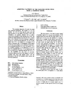
Figure 4: Three examples of density estimation: one too smooth (blue); one too detailed (green); and one which maximizes the likelihood of the test data (red). semantic feature only consists of a single matrix multiplication and single squashing function per network unit.
4.3
Density Estimation
Having computed the features for each of the images in our collection, we perform non-parametric density estimation in order to derive the probabilities P (fji |t). We compute a one-dimensional probability density for each feature dimension using Parzen’s windows [5]. For each feature (pixel or semantic), we use a Gaussian kernel and perform 10-fold cross validation to find the best kernel width. The goal of this step is to build a model of the data that accurately reflects the underlying probability distribution. We find the kernel variance that defines a likelihood model that best predicts the held-out test data. Figure 4 gives an example of this calculation. The distributions are often bimodal or skewed. The product of these distributions is a simple model of image likelihood as a function of the image features.
5. IMPLEMENTATION 5.1 Dataset We consider the following 20 query terms for our evaluation: baby, beetle, butterfly, carnival, chair, Christmas, CN Tower, coast, Colosseum, flower, forest, Golden Gate Bridge, highway, horse, mountain, sailboat, sheep, Statue of Liberty, sunset, wedding. This list includes objects, landmarks, scenes, events and places. We downloaded nearly 4.8 million public, geotagged Flickr images, all with at least one of the tags listed above. The number of images per category ranged from 3,700 to 683,000 images.
5.2
Pixel Feature Implementation
In this paper, we report the results of experiments using three layers of convolution and max-pooling to analyze each image. The input image is converted to YUV and down-sampled so that the longest side is 158 pixels long. The Y channel is high-pass filtered to remove changes in illumination. After downsampling, filtering and zero padding all image are 140×140 pixels. The filter banks of the first two stages have kernels of size 9×9, and the max-pooling is performed over 4×4 and 5×5 non-overlapping windows at the first and second stage, respectively. The third-stage filters have the same size support as one of the second stage feature maps, and therefore, no pooling is performed there. The number of feature maps is equal to 128 at the first stage, 512 at the second stage and 1024 at the third stage. The final feature vector is 1024-dimensional.
85
We trained our feature extractor with the unsupervised algorithm on natural image patches randomly selected from images downloaded from Flickr, and then validated the parameters of our extractor by testing its performance using the Caltech-256 objectclassification task [7]. This allowed us to fine-tune the architecture of our network and the number of layers and nodes. Note that the Caltech-256 data gave us a separate validation set. However, it is important to build our feature extractor using Flickr images since its style is much less constrained than the Caltech-256 set and Flickr represents a larger dataset. The validation of the parameters proceeded as follows after building the feature extractor as described above: we compute the features for each image of the Caltech-256 dataset; then we train a linear SVM classifier with 30 training samples per class. The average recognition accuracy was equal to 26% which is considered to be a good result — the state-of-the-art is in the mid-thirties [7].
5.3
89:;+