Image Segmentation With Maximum Cuts Slav Petrov University of California at Berkeley
[email protected] Spring 2005
Abstract
mation where correspondence between regions has to be established or higher-level problems such as object recognition where recognition of subparts would benefit from good segmentation algorithms. Many different approaches have been proposed in the past. Data clustering methods have been applied to image segmentation in form of agglomerative and divisive algorithms [9]; also techniques based on mapping image pixels to some feature space [1] have been suggested. Recently a graph theoretic approach has become the most popular and a number of authors have demonstrated good performance on this task using methods that are based on graph cuts [18], [13], [3]. One of the advantages of the graph cut methods is that they can make use of well understood algorithms for graph partitioning and that the graph structure allows the search for a globally optimal solution based on local features. This paper is structured as follows: in the following section we will review some related work and then our approach will be described in section three. In section four some results will be shown, before concluding in section six..
This paper presents an alternative approach to the image segmentation problem. Similar to other recent proposals a graph theoretic framework is used: Given an image a weighted undirected graph is constructed, where each pixel becomes a vertex of the graph and edges measure a relationship between pixels. Our approach differs from previous work in the way we define the edge weights. Typically the edge weights represent pixel similiarities and a good segmentation corresponds to a (normalized) minimum cut of the graph. The shortcoming of the minimum cut approach is that it favors cutting small regions of isolated nodes and therefore a normalization is needed in order to enforce a more balanced partitioning. We propose to fix this shortcoming by using a maximum cut approach, because a maximum cut is usually achieved when the clusters are of similar size. Our edge weights measure the pixel dissimilarity and hence we seek a maximum cut of the graph. Since computing the maximum cut is NP-complete we use an approximation algorithm based on semidefinite programming to obtain a good cut. We define different graph structures that can be used and show that the computational complexity of the problem significantly depends on the structure of the graph. Synthetic and real images are segmented and the results are compared to results obtained by alternative segmentation algorithms.
2. Related Work In the graph theoretic framework image segmentation is performed by repeatedly partitioning a graph G = (V, E) into two disjoint sets A and B (A ∪ B = V, A ∩ B = ∅). Given an image I a weighted undirected graph G = (V, E) is constructed, where each pixel becomes a vertex of the graph. The graph is usually fully connected and the edge weight w(i, j) is computed by a function measuring the similarity between the vertices i and j. Low-level features such as brightness, color and texture are typically used for estimating the similarity. Segmenting the image corresponds to finding a partition of the graph into disjoint sets V1 , V2 , V3 , ..., Vm , such that the similarity within the set Vi is high and between two different sets Vi and Vj is low. The objective function for measuring the similarity is where the various approaches differ. The objective function also determines the complexity of the algorithm: in simple cases the complexity is a low de-
1. Introduction Image segmentation (also referred to as perceptual grouping) is one of the most studied and yet unsolved problems in computer vision. The objective is to partition the image into regions of similar appearance and thereby achieve a compact, summary representation [5]. While pixels in the same region should look alike, pixels in different regions should inhibit different low-level features (e.g. color, brightness, texture). The Gestalt movement in psychology [17] showed that perceptual grouping plays an important role in human visual perception and a wide range of computer vision problems could benefit from well segmented images. Examples are intermediate-level vision problems such as stereo esti1
x x x x x x x xx x x x x x x x x x x x
x
x x
x
Min-Cut 2 x
x x
within the groups simultaneously. Unfortunately this more general formulation comes at a high price: computing the optimal normalized cut is NP-complete (as proven by Papadimitriou, see the appendix of [13]) and therefore approximation algorithms need to be applied. It can be shown that computing the eigenvectors of the affinity matrix (which is essentially the adjacency matrix of the graph) produces an approximate solution to the normalized cut problem [13]. Eigenvector based segmentation is used for finding efficiently approximate solutions in the normalized cuts framework, but has also been proposed by others. All these methods find one or several eigenvectors of an affinity matrix and differ only in the way the affinity matrix is defined and how many and which eigenvectors are used. A good overview is presented by Y. Weiss in [16] where different eigenvalue based approaches are compared and analyzed.
x
Min-Cut 1 x
x
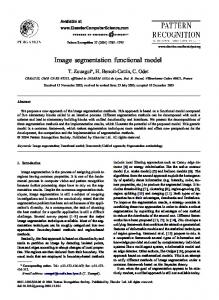
Better Cut Figure 1: The minimum cut favors cutting small sets of isolated nodes (image based on [13]).
3. The Maximum Cut Approach
gree polynomial, but often the computation of an exact solution turns out to be NP-complete; in these cases approximate solutions, often based on eigen-decomposition of the affinity matrix, have been suggested.
Graph partitioning techniques that minimize some objective function have been studied extensively and all kinds of objective functions have been suggested. All of these approaches have to deal with minimum cut’s behavior of favoring small isolated regions. In this paper an alternative approach is pursued: instead of computing a minimum cut, we will compute the maximal cut on an appropriately defined graph. We are interested in partitions where the within cluster similarity is large and the between cluster similarity is small. In the minimum cut framework the edge weights represent the similarity between pixels. One can think of the edges as rubber bands holding the vertices together, with thicker rubber bands holding together more similar pixels. The minimum cut is the one which requires the least energy for cutting the rubber bands and separating the graph in two pieces. In contrast, in the maximum cut framework, the edge weights represent the dissimilarity between pixels. Think of the edges as springs pushing apart pixels that do not look alike. The graph cannot expand arbitrarily but has to fit within a certain size (the image canvas), and therefore the springs have to be compressed, which requires energy. The maximum cut removes the most resisting edges and thereby minimizes the required energy. Finding the maximum cut fixes the shortcoming of minimum cut: the cost of the cut is maximized when there are as many connections as possible, which encourages a partition with larger regions. Maximum cuts are usually used in the electronic circuit design. Given an electronic circuit specified by a graph, the maximum cut defines the largest amount of data communication that can simultaneously take place in the circuit. The highest-speed communications channel should thus span the vertex partition defined by the maximum edge cut. Finding the maximum cut in a graph is
2.1 Minimum Cuts In the framework of minimum cuts the partitioning, also called a cut, is achieved by removing all edges between the two sets. For each cut a cost is defined as follows: X cut(A, B) = w(u, v). u∈A,v∈B
The optimal cut can be computed efficiently with the Ford Fulkerson algorithm [4] and Wu and Leahy [18] show a clustering method based on this minimum cut criterion. However, as the authors themselves mention in their work, this criterion tends to favor cutting small sets of isolated nodes in the graph, see fig. 1.
2.2 Normalized Cuts In order to avoid this unnatural bias Shi and Malik [13] propose a normalized cut (N cut) criterion that measures the within group similarity as well as the cluster dissimilarity and thereby produces better results. It is defined as a fraction of the total edge connections to all nodes in the graph: cut(A, B) cut(A, B) + , assoc(A, V ) assoc(B, V ) P where assoc(A, V ) = u∈A,v∈V w(u, v) is the weight of all edges from nodes in A to all nodes in the graph. As it turns out, this definition allows to minimize the disassociation between the groups and to maximize the association N cut(A, B) =
2
NP-complete, despite the existence of algorithms for minimum cut (MAXCUT is one of Karp’s original NP-complete problems [10]). However, there exist good approximation algorithms.
• Brightness: When working with gray-level images brightness replaces color. But it should be noted that brightness is not a reliable cue when shadows are present (which is essentially always the case).
3.1 Constructing the Graph
• Texture: Probably the best cue is texture. Texture can be measured by the response of DOOG filters at various scales and orientations [11].
The first step consists of constructing an undirected graph based on the given image. There are two independent steps involved: first we need to decide on the graph structure and then we need to compute the edge weights.
• Spatial Proximity: Pixel that are closer to each other in the image are more likely to belong to the same region. This simple fact is measured by the Euclidian distance between the pixel locations in image coordinates.
3.1.1 Graph Structure
• Number of edges between pixels: Edges often coincide with object boundaries. We compute the edge map of the image (using a Canny edge detector) and then count the number of edges that intersect the line between the pixels.
For each image pixel there is a vertex in the graph and the edge weights represent the dissimilarity between two pixels. We experimented with three different approaches for the number of edges in the graph: • Fully connected graph: For each pair of pixels a dissimilarity measure is computed. This graph captures the global dissimilarity between different regions very well, but even for medium sized images (e.g. 1 Megapixel) this approach becomes intractable (the graph will have one million vertices and one trillion edges). Therefore a threshold distance dthresh has to be chosen and only pixels that are at most dthresh apart are connected to each other. Typically dthresh is in the range of 10 to 20 pixels.
We use a weighted average of these features as the dissimilarity measure. Our implementation makes use of The Berkeley Segmentation Engine (BSE) implemented by C. Fowlkes and publicly available at [6].
3.2 Finding the Maximum Cut After the graph has been constructed we want to repeatedly bipartition it by finding maximum cuts. Karp showed by reducing from a slight variant of 3SAT that finding the maximum cut is NP-complete [10]. Since we are working with very large graphs, computing the exact solution is impossible. Instead we either try to find an approximate solution or to restrict the graph to having a planar structure. Depending on the graph one of the following maximum cut algorithms is used for bipartitioning:
• 4- or 8-neighbors graph: This graph captures the local dissimilarities and reduces the number of edges by an order of magnitude. Additionally the neighborhood graph is planar and there exist polynomial time algorithms for finding the maximum cut for planar graphs [8]. Unfortunately some information about global characteristics is lost. • Randomly sampled graph: For each vertex we pick randomly a number of different vertices (20 or 50) and compute the dissimilarity to those. While this graph has a small number of edges it captures hopefully enough local and global information.
3.2.1 A naive greedy algorithm For a long time no good polynomial time approximation algorithm was known. The only solution was a naive greedy algorithm that guarantees a 12 approximation. The idea is to start with any arbitrary cut and then to adjust the nodes a little bit in the following fashion: If some node has more neighbors on its side than on the other side, then move it to the other side. This process is repeated until convergence. Alternatively, a simple randomized algorithm just puts each node on a random side. Every edge has a probability of 12 of crossing cut, hence the expected number of edges crossing the cut is |E| 2 .
In order to further reduce the number of edges we use a sparse representation and remove edges that have a weight smaller than a certain threshold. 3.1.2 Edge Weights Different low-level features can be used for computing the dissimilarity between two pixels: • Color: When working with color images, color obviously is an important grouping indicator. The dissimilarity can be computed for example as the Euclidian distance in the HSV color space.
3.2.2 Approximation algorithms The best known, and probably the best possible, approximation algorithm for maximum cuts is due to M. Goemans and 3
(a)
(b)
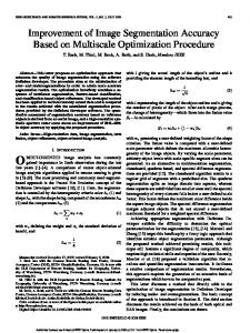
(c)
Figure 2: Segmentation results on a synthetic image that was subsampled to 32x32 pixels: (a) Original image; (b) Normalized cuts segmentation; (c) Our maximum cut result. See text for discussion.
3.3 The Recursive Algorithm
D. Williamson [7] and guarantees to deliver a solution that is at least within a factor of 0.879 of the optimal solution. The algorithm can be interpreted as a semidefinite program or as an eigenvalue minimization problem. The maximum cut of a graph G = (V, E) with weights wij = w(i, j) is given by the following integer program: max
X
After the graph has been partitioned we need to decide whether the current partition is sufficient or whether some components should be recursively subdivided. This is currently done manually, a good stopping criteria is a possible area of future research.
wij (1 − yi yj )
4. Results
(i,j)∈E
In this section we will present and discuss some of the obtained results. It should be noted that, in general, the evaluation of different grouping algorithms is challenging and not well understood since the granularity of the segmentation depends heavily on the application. While there exists databases of human segmented images that can be used as ground truth ([12]),a universally accepted test bench has yet to be established. A common way to present segmentation results is therefore to segment several test images and compare these to segmentations obtained by alternative algorithms. We are showing our segmentation of a synthetic image (fig. 2) and a real image (fig. 3) and are comparing our results to the segmentations produced by J. Shi’s et al. normalized cuts [13], obtained by the implementation that is available at [2]. Unfortunately only results on small images can be shown since the memory requirements for big images are enormous (especially when the code is not optimized). Our maximum cut algorithm was somewhat slower than the normalized cut algorithm, however our code is not optimized. The memory requrements were what prohibited the segmentation of larger images. We are showing results on two images that are realatively easy to segment. For more complicated images our algorithm failed to produce a good segmentation.
subject to: yi ∈ {−1, 1} where the yi are labels indicating to which set each vertex belongs. This integer program can be relaxed so that an approximate solution can be found in polynomial time. The idea is to solve a semidefinite program and then to ”round” the solution appropriately. The ”rounding” is achieved by picking a random hyperplane that separates the solutions of the semidefinite program. See [7] for details. We used a semidefinite programming package for MATLAB called SDP T 3 , which is publicly distributed at [15]. 3.2.3 Algorithms for planar graphs When the underlying graph structure is restricted to be planar the maximum cut can be found by a polynomial time algorithm that is due to Hardlock [8]. Hardlock’s algorithm transforms the maximum cut problem into the maximum weighted matching problem and requires O(n3 ) time. Recently a better algorithm, running in O(n1.5 log n) time, has been developed [14]. Due to time constraints we were not able to implement any of these algorithms for planar graphs but had to use Goemans’ and Williamson’s [7] approximation algorithm for arbitrary graphs. 4
(a)
(b)
(c)
Figure 3: Segmentation results on a real image that was subsampled to 32x32 pixels: (a) Original image; (b) Normalized cuts segmentation; (c) Our maximum cut result. See text for discussion.
References
As can be seen in fig.2 and fig.3 the maximum cut segmentation is not quite as good as the normalized cut, but it is still a sensible grouping. It should be noted that the images were subsampled to 32x32 pixels and then smoothed in order to remove color dithering artifacts, thereby blurring the details inside the wheel. It has not been resolved why the segmentation in 2(c) is not symmetric, but this is the best result that could be obtained (possibly there is bug somewhere). The results shown here were achieved when using a fully connected graph with a maximum distance of dthresh = 10 between connected pixels. There was not enough time for a thorough analysis of the maxcut’s performance depending on different graph structure, but it can be assumed that the results for the other graph structures will be worse. The question would be whether the trade-off between computational cost and segmentation quality is acceptable.
[1] D. Comaniciu and P. Meer. Robust analysis of feature spaces: color image segmentation. In IEEE Conference on Computer Vision and Pattern Recognition, pages 750–755, 1997. [2] T. Cour, S. Yu, and J. Shi. Matlab normalized cuts segmentation code. 2004. http://www.cis.upenn.edu/ jshi/software/. [3] P. Felzenszwalb and D. Huttenlocher. Efficient graph-based image segmentation. International Journal of Computer Vision, 59(2):167–181, 2004. [4] L. Ford and D. Fulkerson. Flows in Networks. Princeton University Press, 1962. [5] D. Forsyth and J. Ponce. Computer Vision: A Modern Approach. Prentice-Hall, Englewood Cliffs, NJ, 2002. [6] C. Fowlkes. The Berkeley Segmentation Engine (BSE). http://www.cs.berkeley.edu/ fowlkes/BSE/. [7] M. Goemans and D. Williamson. Improved approximation algorithms for maximum cut and satisfiability problems using semidefinite programming. In 26th Symposium on the Theory of Computing, pages 422–431, 1994.
5. Summary and Conclusions We introduced an alternative graph theoretic approach to image segmentation. By using pixel dissimilarities as edge weights and finding the maximum cut in the graph we are able to obtain a more balanced cut than with an (unnormalized) minimum cut. While our algorithm produces sensible segmentations, it cannot compete with state of the art algorithms such as normalized cuts [13]. Nonetheless it is interesting from a theoretical point of view and provides some insight into the graph theoretic image segmentation domain.
[8] F. Hardlock. Finding the maximum cut of a planar graph in polynomial time. In SIAM Journal on Computing, pages 221–225, 1975. [9] A. Jain and R. Dubes. Algorithms for Clustering Data. Prentice-Hall, Englewood Cliffs, NJ, 1988. [10] R. Karp. Reducibility among combinatorial problems. In Complexity of Computer Computations, pages 85–103, 1972. [11] J. Malik and P. Perona. Preattentive texture discrimination with early vision mechanisms. Journal Optical Soc. Am., 7(2):923–932, 1990.
Acknowledgments
[12] D. Martin, C. Fowlkes, D. Tal, and J. Malik. A database of human segmented natural images and its application to evaluating segmentation algorithms and measuring ecological statistics. In Proc. 8th Int’l Conf. Computer Vision, volume 2, pages 416–423, July 2001.
Thanks to C. Fowlkes for providing The Berkeley Segmentation Engine (BSE) code [6] and even compiling and setting it up. 5
[13] J. Shi and J. Malik. Normalized cuts and image segmentation. IEEE Transactions on Pattern Analysis and Machine Intelligence, 20(8):888–905, 2000. [14] W. Shih, S. Wu, and Y. Kuo. Unifying maximum cut and minimum cut of a planar graph. IEEE Trans. Computers, 39(5):694–697, 1990. [15] K.-C. Toh, M. Todd, and R. Tutuncu. SDPT3 - a Matlab software package for semidefinite programming, version 3.02. 1997. http://www.math.cmu.edu/ reha/sdpt3.html. [16] Y. Weiss. Segmentation using eigenvectors: a unifying view. In IEEE International Conference on Computer Vision, pages 975–982, 1999. [17] M. Wertheimer. A Sourcebook of Gestalt Psychology. Harcourt, Brace and Company, 1938. [18] Z. Wu and R. Leahy. An optimal graph theoretic approch to data clustering: Theory and its application to image segmentation. IEEE Transactions on Pattern Analysis and Machine Intelligence, 15(11):1,101–1,113, 1993.
6