Image Structure-Preserving Denoising Based on Difference Curvature ...

Hindawi Publishing Corporation Mathematical Problems in Engineering Volume 2015, Article ID 930984, 16 pages http://dx.doi.org/10.1155/2015/930984

Research Article Image Structure-Preserving Denoising Based on Difference Curvature Driven Fractional Nonlinear Diffusion Xuehui Yin1,2 and Shangbo Zhou1,2 1

Key Laboratory of Dependable Service Computing in Cyber Physical Society of Ministry of Education, Chongqing University, Chongqing 400030, China 2 College of Computer Science, Chongqing University, Chongqing 400030, China Correspondence should be addressed to Shangbo Zhou; [email protected] Received 17 November 2014; Revised 17 March 2015; Accepted 17 March 2015 Academic Editor: Muhammad N. Akram Copyright © 2015 X. Yin and S. Zhou. This is an open access article distributed under the Creative Commons Attribution License, which permits unrestricted use, distribution, and reproduction in any medium, provided the original work is properly cited. The traditional integer-order partial differential equations and gradient regularization based image denoising techniques often suffer from staircase effect, speckle artifacts, and the loss of image contrast and texture details. To address these issues, in this paper, a difference curvature driven fractional anisotropic diffusion for image noise removal is presented, which uses two new techniques, fractional calculus and difference curvature, to describe the intensity variations in images. The fractional-order derivatives information of an image can deal well with the textures of the image and achieve a good tradeoff between eliminating speckle artifacts and restraining staircase effect. The difference curvature constructed by the second order derivatives along the direction of gradient of an image and perpendicular to the gradient can effectively distinguish between ramps and edges. Fourier transform technique is also proposed to compute the fractional-order derivative. Experimental results demonstrate that the proposed denoising model can avoid speckle artifacts and staircase effect and preserve important features such as curvy edges, straight edges, ramps, corners, and textures. They are obviously superior to those of traditional integral based methods. The experimental results also reveal that our proposed model yields a good visual effect and better values of MSSIM and PSNR.

1. Introduction A challenging task in designing image denoising model is to retain significant features, such as edges and texture details, while eliminating noise. Among a variety of integer-order partial differential equations based image denoising techniques [1–3], energy minimization based variational technique in two well-known forms of the nonlinear diffusion with anisotropic diffusion proposed by Perona and Malik [4] (Perona-Malik or PM) and total variation (TV) regularization proposed by Rudin et al. [5] (Rudin-Osher-Fatemi or ROF) are the ones that have shown a good edge preservation capability. Most of these nonlinear diffusion models are developed from the following model: 𝜕𝑢 − ∇ ⋅ (𝜑 (𝑥, 𝑦) ∇𝑢) = 0, 𝜕𝑡

(1)

by changing the form of 𝜑(𝑥, 𝑦), which decides the degree of denoising and preservation of singularities (e.g., noise, edges,

and texture). The isotropic diffusion expressed by a linear heat equation has been replaced by the anisotropic diffusion since the classical model was proposed by Perona and Malik in 1990. It is well known that the PM model yields very favorable results for eliminating image noise while retaining object edges and reducing oscillations. However, it also possesses some unsatisfactory properties in some cases; that is, it easily loses the contrast and texture details and produces staircase effects and so on [6, 7]. To remedy the loss of contrast and texture details, some scholars proposed an iterative regularization method for image restoration [8], and 𝐿2 norm in the fidelity term in (1) was replaced by 𝐿1 norm in [9– 12]. Staircase effect is one of the unsatisfactory properties of the PM model. On the other hand, in [13–17], some models for image noise removal have been introduced to prevent staircase effect, which are based on higher order derivatives to energy norm or integrate high-order derivatives to original model. In addition, a total generalized variation (TGV)

2

Mathematical Problems in Engineering

[18, 19] has been presented, which contains order greater than or equal to 2, unlike TV, which only considers first-order derivatives. It has some effects on image denoising, which not only leads to piecewise polynomial intensities but also obtains almost perfect edges while efficiently avoiding staircase effect. Recently, geometric attributes of images have been incorporated into the image denoising processing. The most commonly used local geometrical features are the curvature of the image level curve [20, 21], the Gauss curvature of the image surface [22–25], and the mean curvature of the image surface [26]. Although the aforementioned models have some effects on retaining image contrast, textures, and removing staircase effects, the results are still unsatisfactory. In short, the previously proposed models are integer-order differential based model in essence, they may produce blur edges, and their effect for textures preservation is not well. In particular, the variational method based high-order derivatives of the denoised image often lead to speckle artifacts, that is, isolated black and white speckles. Thus, in order to preserve textures and achieve a good tradeoff between eliminating speckle artifacts and restraining staircase effect, as a compromise between second-order PDEs and high-order PDEs, fractional-order PDEs based methods have been investigated and applied in the fields of computer vision. Unlike our familiar derivative operator, that is the integer-order derivative operator, the fractional-order derivative operator expands the integer-order derivative operator; it possesses the “nonlocal” property because the fractionalorder derivative at a point depends upon the characteristics of the entire function and not just the values in the vicinity of the point [27–30], which is beneficial to improve the performance of textures preservation. Bai and Feng (BF) [31] present an anisotropic diffusion equation based on fractional-order space derivatives for image denoising. Their proposed model is interpolated between the PM equation and the fourth-order anisotropic diffusion equation, which is modeled by 𝜕𝑢 ∗ 󵄨 󵄨2 = −𝐷𝑥𝛼 (𝑐 (󵄨󵄨󵄨𝐷𝑥𝛼 𝑢󵄨󵄨󵄨 ) 𝐷𝑥𝛼 𝑢 (𝑥, 𝑦)) 𝜕𝑡 −

∗ 𝐷𝑦𝛼

󵄨 󵄨2 (𝑐 (󵄨󵄨󵄨󵄨𝐷𝑦𝛼 𝑢󵄨󵄨󵄨󵄨 ) 𝐷𝑦𝛼 𝑢 (𝑥, 𝑦)) , ∗

∗

(2)

where 𝑐(𝑠) = 1/(1 + 𝑠) and 𝐷𝑥𝛼 and 𝐷𝑦𝛼 are the adjoints of 𝐷𝑥𝛼 and 𝐷𝑦𝛼 , respectively. The numerical results implemented fractional developmental equation in frequency domain and showed that both of the staircase effect and the speckle artifacts can be eliminated effectively. Guidotti and Lambers [32] extended gradient operator of energy norm from first-order to fractional-order. It has some effects on image denoising. Zhang et al. [33, 34] generalized the classical integer-order TV regularization model for image denoising, which is based on the Gr¨unwald-Letnikov fractional-order derivative. Numerical examples show that the new models can eliminate both staircase effect and speckle artifacts when the parameters are chosen appropriately. Moreover, they are able to retain textures better than the TV model. For the case of calculation, Pu et al. [35] scheduled a class of fractional-order differential masks and illustrated that fractional-order differentiation can

handle well fine structures such as texture. With regard to the tomographic reconstruction of the blurry and noisy binary images, a variational approach based on adapted fractionalorder Hilbert spaces has been proposed by Bergounioux and Tr´elat [36]. A class of fully fractional anisotropic diffusion models was presented by Janev et al. [37] for noise removal, where spatial as well as time fractional-order derivatives are employed. Cuesta et al. [38] deduced a Volterra matrix-valued equation for image noise removal from a generalization of the linear fractional integral equation. However, they still have many great potential drawbacks. They simply used the first-order gradient operator of the energy norm to displace fractional-order one and the algorithms do not consider the fractional power of the energy norm, so the loss of image contrasts is not kept well after denoising. In this paper, we aim to use two new techniques, fractional calculus and difference curvature to image denoising. In comparison to the Gauss curvature and the mean curvature, the difference curvature can more effectively distinguish between ramps and edges. The fractional-order derivatives are able to better deal with the textures of the image and achieve a good tradeoff between eliminating speckle artifacts and restraining staircase effect on the entire image. We combine the difference curvature and fractional calculus frames for one diffusion. Near object edges, the difference curvature is large and the total variation term approximates to the 𝐿1 norm of fractional-order gradient flow for the image in order to preserve the edges; away from the edges (in ramp and flat regions), the difference curvature is small and the total variation term approximates to the 𝐿2 norm of fractional-order gradient flow for the image in order to prevent staircase effect. It is confirmed that the difference curvature is able to distinguish effectively between ramps and edges. Therefore the proposed model can effectively distinguish between ramps and edges, while improving the performance of texture preservation and preventing staircase effect and speckle artifacts. The remainder of this paper is organized as follows. In Section 2, the fractional-order derivatives and the new edge indicator (difference curvature) are briefly reviewed. In Section 3, based on fractional-order derivatives and the difference curvature the proposed model and algorithm are presented. Section 4 develops a numerical algorithm to implement our proposed model. Section 5 is devoted to experimental examples. Comparing the simulation results obtained by our proposed denoising model with the baseline denoising methods reports a noticeable improvement in the quality of the denoised images evaluated qualitatively and quantitatively. Section 6 is a conclusion.

2. Preliminaries 2.1. Fractional-Order Derivatives. As a generalization form of the integer-order derivative, the fractional-order derivative has a long history, but it has no uniform definition until now. Three class definitions, Gr¨umwald-Letnikov definition, Riemann-Liouville definition, and Caputo definition [29],

Mathematical Problems in Engineering

3

are generally carried out by some investigations in recent literatures. Let us introduce the representation of an 𝑛-fold integral 𝐽𝑛 for 𝑓 ∈ 𝐿1 ([0, +∞]) as follows: 𝐽𝑛 𝑓 (𝑡) =

𝑡 1 ∫ (𝑡 − 𝜏)𝑛−1 𝑓 (𝜏) 𝑑𝜏. (𝑛 − 1)! 0

(3)

Replacing 𝑛 ∈ N in (3), we obtain a definition of a fractionalorder integral 𝑡 1 𝐽 𝑓 (𝑡) = ∫ (𝑡 − 𝜏)𝛼−1 𝑓 (𝜏) 𝑑𝜏, Γ (𝛼) 0 𝛼

a new feature descriptor called difference curvature (DC). We define 󵄨󵄨 󵄨 󵄨 󵄨󵄨 (9) DC = 󵄨󵄨󵄨󵄨󵄨󵄨󵄨󵄨𝑢𝜂𝜂 󵄨󵄨󵄨󵄨 − 󵄨󵄨󵄨󵄨𝑢𝜉𝜉 󵄨󵄨󵄨󵄨󵄨󵄨󵄨󵄨 , where 𝑢𝜂𝜂 and 𝑢𝜉𝜉 represent the second-order derivatives in the direction of the gradient ∇𝑢 and in the direction perpendicular to ∇𝑢, respectively, and the operator |⋅| denotes the absolute value. Here 𝑢𝜂𝜂 =

𝑢𝑥2 𝑢𝑥𝑥 + 2𝑢𝑥 𝑢𝑦 𝑢𝑥𝑦 + 𝑢𝑦2 𝑢𝑦𝑦 𝑢𝑥2 + 𝑢𝑦2

0 < 𝑡 < +∞, (4)

where Γ(𝛼) is Euler’s continuous gamma function. In particular, if 𝛼 ∈ N, then Γ(𝛼) = (𝛼 − 1)!. Let 𝑛 = [𝛼], the operator 𝐷𝛼 defined as 𝐷𝛼 𝑓 (𝑡) = 𝐷𝑛 𝐽𝑛−𝛼 𝑓 (𝑡)

(5)

for 0 < 𝑡 < +∞ is called the Riemann-Liouville (R-L) differential operator with order 𝛼. However, in this paper, we apply the frequency domain definition to extend the step from integer to fractional, because it is easier for calculating. Therefore, the fractional-order partial derivatives can be formulated as 𝐷𝑥𝛼 𝑢 (𝑥, 𝑦) =

1 𝛼 ̂ (𝜔1 , 𝜔2 ) 𝑑𝜔1 𝑑𝜔2 , ∫ 𝑒𝑖(𝑥𝜔1 +𝑦𝜔2 ) (𝑖𝜔1 ) 𝑢 2 2𝜋 R

𝐷𝑦𝛼 𝑢 (𝑥, 𝑦) =

1 𝛼 ̂ (𝜔1 , 𝜔2 ) 𝑑𝜔1 𝑑𝜔2 . ∫ 𝑒𝑖(𝑥𝜔1 +𝑦𝜔2 ) (𝑖𝜔2 ) 𝑢 2𝜋 R2 (6)

It is natural that the 2D fractional-order gradient operator is able to be formulated as 𝐷𝛼 𝑔(𝑥, 𝑦) = (𝐷𝑥𝛼 𝑔, 𝐷𝑦𝛼 𝑔), with the associated magnitude |𝐷𝛼 𝑔| = √(𝐷𝑥𝛼 𝑔)2 + (𝐷𝑦𝛼 𝑔)2 . The definition of fractional-order Hilbert space 𝐻𝑠 (R𝑛 ) goes by using the Fourier transform as follows [31, 36]. For arbitrary number 𝑠 > 0, define 󵄨 󵄨2 𝑠/2 ̂ 𝐻𝑠 (R𝑛 ) = {𝑓 ∈ 𝐿2 (R𝑛 ) | (1 + 󵄨󵄨󵄨𝜉󵄨󵄨󵄨 ) 𝑓 (𝜉) ∈ 𝐿2 (R𝑛 )} (7) endowed with the norm 1/2 󵄩󵄩 󵄩󵄩 󵄨 󵄨2 𝑠 󵄨 ̂ 󵄨󵄨󵄨2 (𝜉)󵄨󵄨 𝑑𝜉) , 󵄩󵄩𝑓󵄩󵄩𝐻𝑠 (R𝑛 ) = (∫ (1 + 󵄨󵄨󵄨𝜉󵄨󵄨󵄨 ) 󵄨󵄨󵄨󵄨𝑓 R𝑛

(8)

̂ where 𝑓(𝜉) is the Fourier transform of 𝑓(𝜉). We denote by 𝐻𝑠 (Ω)∗ the dual of 𝐻𝑠 (Ω). 2.2. Difference Curvature. It is generally appreciated that the gradient of an image cannot effectively distinguish between the image edges and the image ramps. It is well known that the second-order derivatives are able to effectively distinguish edges and ramps in the case of one-dimensional signal [14]. Similarly, in the two-dimensional case of images, in order to effectively distinguish edges and ramps, we will introduce

𝑢𝜉𝜉 =

𝑢𝑦2 𝑢𝑥𝑥 − 2𝑢𝑥 𝑢𝑦 𝑢𝑥𝑦 + 𝑢𝑥2 𝑢𝑦𝑦 𝑢𝑥2 + 𝑢𝑦2

, (10) .

The value of DC is large at the object edges, while it is small in flat and ramp regions [39], so the edges can be distinguished from flat and ramp regions when the DC is computed for an image. The property analysis of the new feature descriptor is as follows. (a) At image edges, |𝑢𝜂𝜂 | is large and |𝑢𝜉𝜉 | is small, so DC is large. (b) In flat and ramp regions, |𝑢𝜂𝜂 | and |𝑢𝜉𝜉 | are both small, so DC is small. (c) At isolated noise, |𝑢𝜂𝜂 | and |𝑢𝜉𝜉 | are both large but they are almost equal, so DC is small.

3. Difference Curvature-Based Fractional Anisotropic Diffusion Model 3.1. Description of Our Proposed Model. Let us recall a classic example of noise removal scheme driven by curvature, which is an isotropic diffusion scheme, where the smoothing process is formulated by a partial differential equation. Let 𝑢 denote an image intensity function, 𝑡 is the time (scale parameter), and 𝑐(⋅) denotes the speed function which is dependent on the curvature 𝜅 of the level curve; then the diffusion equation can be formulated as 𝜕𝑢 (11) = 𝑐 (𝜅) |∇𝑢| . 𝜕𝑡 If 𝑐(𝜅) = 𝜅, (11) is the standard curvature evolution equation [21]. With introducing a new coordinate 𝑧 and assigning the grey level of the image to the coordinate, we obtain a level function 𝜓(𝑥, 𝑦, 𝑧) = 𝑢(𝑥, 𝑦) − 𝑧. Then the image 𝑢(𝑥, 𝑦) can be viewed as its zero level set {(𝑥, 𝑦, 𝑧) : 𝜓(𝑥, 𝑦, 𝑧) = 0} corresponds to the surface 𝑧 = 𝑢(𝑥, 𝑦). In [23], the mean curvature of image surface evolution for noise removal is proposed, which is modeled by 𝜕𝑢 =∇⋅( 𝜕𝑡 √

1 1 + |∇𝑢|2

∇𝑢) (12)

=∇⋅(

1 √1 + 𝑢𝑥2 + 𝑢𝑦2

∇𝑢 (𝑥, 𝑦)) .

4

Mathematical Problems in Engineering

A modified mean curvature motion for image smooth is proposed in [24]. Chan et al. [25] developed a diffusion equation which uses the mean curvature as the conductance term, that is, the mean curvature driven diffusion (MCDD) in which the amount of diffusion is dependent on the mean curvature, which can be written as 𝜕𝑢 = ∇ ⋅ (𝑀∇𝑢 (𝑥, 𝑦)) , 𝜕𝑡

𝑥

0.7 0.6 0.5 0.3 0.2

(14)

0.1 0 −100 −80 −60 −40 −20

0

20

0

60

80

100

y1 = exp(−(x/k)2 ) y2 = 1/(1 + (x/k)2 ) y3 = exp(−|x|/k)

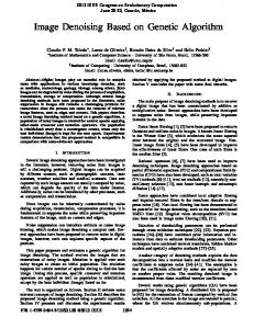
Figure 1: Comparison of three conductance functions.

𝑦

where 𝜙 : R → [0, +∞] is a decreasing and continuous 2 )/(1 + function, 𝜙(|∇𝑢|) ≥ 0 with 𝜙(0) = 0, and (𝑢𝑥𝑥 𝑢𝑦𝑦 − 𝑢𝑥𝑦 𝑢𝑥2 + 𝑢𝑦2 )2 is the Gauss curvature of the image surface 𝑧 = 𝑢(𝑥, 𝑦). It is well known that the mean curvature and the Gauss curvature are the average and product of |𝑢𝜂𝜂 | and |𝑢𝜉𝜉 |, respectively, which can be defined as 󵄨󵄨 󵄨󵄨 󵄨󵄨 󵄨󵄨 󵄨󵄨𝑢𝜂𝜂 󵄨󵄨 + 󵄨󵄨𝑢𝜉𝜉 󵄨󵄨 MC = 󵄨 󵄨 󵄨 󵄨 , 2

0.8

0.4

(13)

where 𝑀 is the mean curvature. Lee and Seo [26] proposed a Gauss curvature driven diffusion (G-CDD) model in which the amount of diffusion is determined by the Gauss curvature; that is, 2 𝑢𝑥𝑥 𝑢𝑦𝑦 − 𝑢𝑥𝑦 𝜕𝑢 ) ∇𝑢 (𝑥, 𝑦)) , = ∇ ⋅ (𝜙 ( 2 𝜕𝑡 (1 + 𝑢2 + 𝑢2 )

1

0.9

GC = 𝑢𝜂𝜂 ⋅ 𝑢𝜉𝜉 ,

propose a novel diffusion model for image denoising which uses the difference curvature in the conductance term to describe the intensity variations in images, which is named difference curvature driven fractional-order anisotropic diffusion (DCFAD) and modeled by 𝜕𝑢 ∗ = −𝐷𝑥𝛼 (𝜙 (DC) 𝐷𝑥𝛼 𝑢 (𝑥, 𝑦)) 𝜕𝑡

(15)

where MC is mean curvature and GC is Gauss curvature. Let us discuss the performance comparisons of gradient and three curvatures, that is, mean curvature, Gauss curvature, and difference curvature. Compared with the flaw of anisotropic diffusion which has a tendency to estimate the false edges during the evolution, the difference curvature driven diffusion for images is more appropriate than the gradient driven diffusion to detect the intensity oscillations because the difference curvature can distinguish the edges and ramp regions; however the gradient difference between edges and ramps is not significant. Although the mean curvature and the difference curvature can effectively distinguish edges and ramps, the mean curvature cannot distinguish edges and isolated noise in a noisy image. For the Gaussian curvature, especially when the image is with isolated noise, the values at corners are large, so the denoising based on the Gaussian curvature driven diffusion cannot retain corners. Meanwhile, the gradient and three curvatures both have a flaw of forming piecewise constant images and indistinctness of texture details because they use the integer-order derivative. Inspired by fractional-order anisotropic diffusion and the (mean/Gauss) curvature driven diffusion by introducing fractional calculus instead of the (mean/Gauss) curvature, we

− ∗

∗ 𝐷𝑦𝛼

(16)

(𝜙 (DC) 𝐷𝑦𝛼 𝑢 (𝑥, 𝑦)) ,

∗

where 𝐷𝑥𝛼 and 𝐷𝑦𝛼 are the adjoints of 𝐷𝑥𝛼 and 𝐷𝑦𝛼 , respectively, 𝜙(DC) = exp(−DC/𝐾) is conductance (diffusivity) function based on Laplacian kernel [40], and 𝐾 is a threshold constant. As shown in Figure 1, compared with two conductance functions of PM diffusion model, the diffusion speed of conductance function based on Laplacian kernel is between them at object edges (where DC is large), and it is smaller than them in flat and ramp regions (where DC is large).

4. Numerical Implementation In this section, to solve (16), we introduce the frequency domain definition for the fractional-order derivative because it is easy to implement. We suppose the original discrete image has 𝑛 × 𝑛 pixels and is uniformly sampled from its continuous version starting at (0, 0). It is a finite and discrete 2D signal, which stands for the actual image pixels in 𝑛 × 𝑛 resolution. We employ the 2D discrete Fourier transform (2D DFT) to approximate the spatial fractional-order difference. Note that we usually handle an image on a bounded domain, while the Fourier domain fractional-order derivative is defined on the whole space. Thus, the image should be prolonged onto the whole space in practical computations.

Mathematical Problems in Engineering

5

Fractional central partial difference formulation (see [31]) can have the following form: ̃ 𝛼 𝑢 = 𝐹−1 ((1 − exp ( −𝑗2𝜋𝜔1 )) 𝐷 𝑥 𝑛

𝛼

−𝑗𝜋𝛼𝜔1 ̂ (𝜔1 , 𝜔2 ) ) , × exp ( )𝑢 𝑛 ̃ 𝛼 𝑢 = 𝐹−1 ((1 − exp ( −𝑗2𝜋𝜔2 )) 𝐷 𝑦 𝑛

(17)

𝛼

−𝑗𝜋𝛼𝜔2 ̂ (𝜔1 , 𝜔2 ) ) , × exp ( )𝑢 𝑛

(18)

To solve (16), the finite difference schemes are applied as follows. Let Δ𝑡 be the time step; we calculate the iterative scheme of the initial image 𝑢(𝑥, 𝑦) and work in the Fourier domain, only returning to the spatial domain when calculating 𝑙𝑥𝑛 = 𝜙(DC)𝐷𝑥𝛼 𝑢𝑛 and 𝑙𝑦𝑛 = 𝜙(DC)𝐷𝑦𝛼 𝑢𝑛 , where 𝜙(DC) = exp(−DC/𝐾). We suppose that the image 𝑢(𝑡) is defined on {1ℎ, 2ℎ, . . . , 𝑁ℎ} × {1ℎ, 2ℎ, . . . , 𝑁ℎ}, where ℎ is the space step size. We 𝑛 𝑛 = 𝑢(𝑛𝜏, 𝑖ℎ, 𝑗ℎ). We denote 𝑢𝑖,𝑗 = 0 for use the notation 𝑢𝑖,𝑗 𝑖, 𝑗 < 1 or 𝑖, 𝑗 > 𝑁. The discrete approximation is defined as follows: 𝑛 𝐷𝑥 𝑢𝑖,𝑗

where 𝜔1 , 𝜔2 ∈ {0, 1, . . . , 𝑛 − 1} are DFT frequencies that correspond to 𝑥 and 𝑦, respectively. 𝐹−1 is the inverse 2D DFT operator. ̃ 𝛼 𝑢 and 𝐷 ̃ 𝛼 𝑢 are calculated by The adjoints of operators 𝐷 𝑥 𝑦 the following formulation, respectively: ̃ 𝛼 𝑢 = 𝐹−1 (conj (1 − exp ( −𝑗2𝜋𝜔1 )) 𝐷 𝑥 𝑛 ∗

× exp ( ∗

× exp (

𝛼

(19)

= (𝐹

−1

−𝑗2𝜋𝜔1 −𝑗𝜋𝛼𝜔1 )) exp ( )) (20) 𝑛 𝑛

∘ 𝐾1 ∘ 𝐹) = 𝐹

∗

∘ 𝐾1 ∘ 𝐹,

(21)

,

ℎ

,

2

2 −1

2

𝑛 𝑛 ) + (𝐷𝑦 𝑢𝑖,𝑗 )) , ⋅ ((𝐷𝑥 𝑢𝑖,𝑗 𝑛

2

𝑛 𝑛 𝑛 𝑛 𝑛 ) 𝐷𝑥𝑥 𝑢𝑖,𝑗 − 2𝐷𝑥 𝑢𝑖,𝑗 𝐷𝑦 𝑢𝑖,𝑗 𝐷𝑥𝑦 𝑢𝑖,𝑗 (𝑢𝜉𝜉 )𝑖,𝑗 = ((𝐷𝑦 𝑢𝑖,𝑗 2

𝑛 𝑛 + (𝐷𝑥 𝑢𝑖,𝑗 ) 𝐷𝑦𝑦 𝑢𝑖,𝑗 ) 2 −1

2

𝑛 𝑛 ) + (𝐷𝑦 𝑢𝑖,𝑗 )) , ⋅ ((𝐷𝑥 𝑢𝑖,𝑗

󵄨󵄨󵄨󵄨 𝑛 󵄨󵄨 󵄨󵄨 𝑛 󵄨󵄨󵄨󵄨 (DC)𝑛𝑖,𝑗 = 󵄨󵄨󵄨󵄨󵄨󵄨(𝑢𝜂𝜂 )𝑖,𝑗 󵄨󵄨󵄨 − 󵄨󵄨󵄨(𝑢𝜉𝜉 )𝑖,𝑗 󵄨󵄨󵄨󵄨󵄨󵄨 . 󵄨 󵄨 󵄨󵄨 󵄨󵄨 Our noise removal method for solving (16) is as follows.

where 𝐾1∗ = diag (conj ((1 − exp (

ℎ

𝑛 𝑛 + (𝐷𝑦 𝑢𝑖,𝑗 ) 𝐷𝑦𝑦 𝑢𝑖,𝑗 )

𝛼

−1

𝑛 𝑛 𝑛 𝑢𝑖,𝑗+1 + 𝑢𝑖,𝑗−1 − 2𝑢𝑖,𝑗

,

2

−𝑗𝜋𝛼𝜔2 ̂ (𝜔1 , 𝜔2 ) ) , )𝑢 𝑛

∗

,

𝑛 𝑛 𝑛 𝑛 𝑢𝑖+1,𝑗+1 + 𝑢𝑖−1,𝑗−1 − 𝑢𝑖+1,𝑗−1 + 𝑢𝑖−1,𝑗+1

𝑛

stands for a diagonal matrix and ∘ represents the matrix mul∗ ̃ 𝛼 𝑢 of 𝐷 ̃ 𝛼 𝑢 is calculated by tiplication. The adjoint operator 𝐷 𝑥 𝑥 the following formulation: ∗ ̃𝛼 𝑢 𝐷 𝑥

ℎ

𝑛 𝑛 𝑛 𝑛 𝑛 (23) (𝑢𝜂𝜂 )𝑖,𝑗 = ((𝐷𝑥 𝑢𝑖,𝑗 ) 𝐷𝑥𝑥 𝑢𝑖,𝑗 + 2𝐷𝑥 𝑢𝑖,𝑗 𝐷𝑦 𝑢𝑖,𝑗 𝐷𝑥𝑦 𝑢𝑖,𝑗

where conj(⋅) is the complex conjugation. ̃ 𝛼 𝑢 has the form 𝐷 ̃ 𝛼 𝑢 = 𝐹−1 ∘ 𝐾1 ∘ 𝐹, where Operator 𝐷 𝑥 𝑥 𝐾1 = diag ((1 − exp (

𝑛 𝑛 𝑢𝑖,𝑗+1 − 𝑢𝑖,𝑗

,

ℎ

𝑛 𝐷𝑦𝑦 𝑢𝑖,𝑗 = 𝑛 = 𝐷𝑥𝑦 𝑢𝑖,𝑗

=

ℎ

𝑛 𝑛 𝑛 𝑢𝑖+1,𝑗 + 𝑢𝑖−1,𝑗 − 2𝑢𝑖,𝑗

𝑛 𝐷𝑥𝑥 𝑢𝑖,𝑗 =

𝛼

−𝑗𝜋𝛼𝜔1 ̂ (𝜔1 , 𝜔2 ) ) , )𝑢 𝑛

̃ 𝛼 𝑢 = 𝐹−1 (conj (1 − exp ( −𝑗2𝜋𝜔2 )) 𝐷 𝑦 𝑛

𝑛 𝐷𝑦 𝑢𝑖,𝑗

=

𝑛 𝑛 𝑢𝑖+1,𝑗 − 𝑢𝑖,𝑗

−𝑗2𝜋𝜔1 𝛼 −𝑗𝜋𝛼𝜔1 )) exp ( ))) . 𝑛 𝑛 (22) 𝛼

𝛼∗

̃ 𝑢. As is proven in ̃ 𝑢 and 𝐷 The same is obtained for 𝐷 𝑦 𝑦 ̃ 𝛼 𝑢 is real [31], when the image size 𝑛 is an odd integer, then 𝐷 𝑥 valued. When 𝑛 is an even integer, the domain of function 𝑝(𝜔1 ) = (1 − exp(−𝑗2𝜋𝜔1 /𝑛))𝛼 is not symmetric with respect to 𝜔1 = [𝑛/2], so usually there is a complex component ̃ 𝛼 𝑢. However, the image size is large enough (e.g., 𝑛 = in 𝐷 𝑥 512, as used in the experiments); this complex component is very small due to the fact that the symmetry is minimally disturbed so that it can be ignored in computations.

Step 1. Let the input image be 𝑢 and set 𝑛 = 1, 𝑢𝑛 = 𝑢, 𝑘, Δ𝑡, ̂ 𝑛 of 𝑢𝑛 . and 𝑡 = 𝑘Δ𝑡; calculate the 2D DFT 𝑢 𝛼

̃ 𝑢𝑛 Step 2. Calculate the 𝛼-order central partial differences 𝐷 𝑥 𝛼 ̃ and 𝐷𝑦 𝑢𝑛 using (18). ̃ 𝛼 𝑢𝑛 and 𝑙𝑦𝑛 Step 3. Calculate 𝑙𝑥𝑛 = 𝜙((DC)𝑛𝑖,𝑗 )𝐷 𝑥 ̃ 𝛼 𝑢𝑛 in the spatial domain. 𝜙((DC)𝑛𝑖,𝑗 )𝐷 𝑦 ̂ = 𝐾∗ ∘ 𝐹(𝑙 ) + 𝐾∗ ∘ 𝐹(𝑙 ). Calculate 𝑑 𝑛

1

𝑥𝑛

2

=

𝑦𝑛

̂ × Δ𝑡 and set 𝑛 = 𝑛 + 1; if ̂𝑛 − 𝑑 ̂ 𝑛+1 = 𝑢 Step 4. Calculate 𝑢 𝑛 ̂ 𝑛 and then stop; else go to 𝑛 = 𝑘, calculate the 2D IDFT of 𝑢 Step 2.

6

Mathematical Problems in Engineering

Table 1: Comparison of the denoising performance for the testing images using different methods with three different values of Gaussian noise standard deviation 𝜎. Results of a consistent PSNR (the first line) and MSSIM (the second line) are listed, respectively. Image

𝜎 10

Barbara (512 × 512)

20 30 10

Bicycle (512 × 512)

20 30 10

Baboon (512 × 512)

20 30

PM 33.08 0.921 30.86 0.861 27.26 0.810 29.13 0.845 24.74 0.723 22.67 0.648 29.12 0.873 24.86 0.743 22.80 0.645

Fourth-order PDEs 33.27 0.923 30.68 0.854 27.89 0.822 29.28 0.851 24.68 0.721 22.81 0.651 29.27 0.876 25.00 0.744 22.85 0.647

ZC 33.52 0.942 31.44 0.901 28.41 0.847 30.32 0.869 26.82 0.781 24.89 0.720 29.89 0.888 25.46 0.768 23.32 0.663

5. Experimental Results To analyze and show the good denoising capability of our proposed difference curvature driven fractional-order anisotropic diffusion (DCFAD) for image denoising, some experiments are carried out to compare the denoising result of the proposed method with that of several baseline denoising methods, including the PDE-based methods, the PM model [4], fourth-order PDEs [13], mean curvature-based variational model proposed by Zhu and Chan (ZC) [22], Gauss curvature driven diffusion (G-CDD) [26], the fractional anisotropic diffusion proposed by Bai and Feng (BF) [31], and the other class methods: nonlocal means filtering (NLMF) [41], the wavelet-based method (Bayes least-squares estimate of Gaussian scale mixture, BLS-GSM) [42], and the total generalized variation (TGV) [19]. The proper selection of the fractional-order 𝛼 of our proposed model depends on the noisy image. We have tested the order from 0.1 to 3.0 with step size of 0.2 on every testing image and we find that 𝛼 = 1.8 can get the best results on the “Barbara” image, 𝛼 = 1.6 can get the best results on the “Bicycle” image, and 𝛼 = 1.8 can get the best results on the “Baboon” image. The time step is set to be Δ𝑡 = 4−𝛼 [35] and 𝐾 = 30. For our model, the peak signal to noise ratio (PSNR) and the mean structural similarity (MSSIM) [43] are adopted to illustrate denoising performance and structure preservation in terms of objective criterion and visual fidelity. We adopt a uniform stopping criterion for all the baseline denoising methods and the proposed method; that is, PSNR(𝑢𝑛+1 ) < PSNR(𝑢𝑛 ) or the iteration counter becomes larger than 5000 otherwise, where 𝑢𝑛 denotes the denoised image in the 𝑛th iteration. The results of all methods are obtained by performing under MATLAB

Denoising methods G-CDD BF NLMF 33.45 34.31 32.58 0.935 0.946 0.909 31.23 31.63 30.42 0.896 0.905 0.851 28.17 29.21 27.65 0.831 0.861 0.815 30.20 30.65 30.26 0.858 0.870 0.866 25.88 27.27 26.05 0.731 0.801 0.777 23.11 25.17 23.14 0.655 0.735 0.656 29.68 30.11 28.99 0.882 0.882 0.831 25.29 25.86 24.48 0.759 0.766 0.607 23.16 23.75 21.13 0.658 0.661 0.456

BLS-GSM 35.06 0.958 32.38 0.917 29.36 0.870 31.10 0.876 27.31 0.808 25.23 0.749 30.18 0.890 26.03 0.773 23.88 0.670

TGV 34.52 0.951 32.08 0.913 29.26 0.863 30.84 0.871 27.30 0.806 25.21 0.742 30.13 0.884 25.96 0.769 23.80 0.664

Proposed 35.79 0.974 32.71 0.926 29.86 0.885 31.62 0.889 27.52 0.826 26.04 0.761 30.26 0.895 26.12 0.780 24.14 0.692

R2011a running on a desktop with Intel Core i3-2120 CUP 3.30 GHz and 8 GB of memory under 64-bit Windows 7. Figure 2 shows the results of comparison of some denoising methods on a digital image “Barbara.” The values of PSNR and MSSIM on image “Barbara” are presented in Table 1. In Figure 2(a), the original image is presented and the noisy image with stand variance 𝜎 = 20 is shown in Figure 2(b). Figures 2(c)–2(g) show the denoising results with the PM model, fourth-order PDEs, ZC, G-CDD, BF, NLMF, BLSGSM, TGV, and our proposed DCFAD model, respectively. In order to perform better than the other models, we present the denoising results of a small patch of the original noisy image in Figure 3. From Figure 3 and Table 1, we can see the following performances. (1) A large scale cartoon part (face) shows staircase effect in the PM model because the flat regions have been smoothed very strongly. (2) The denoising result of the fourth-order PDEs shows speckle artifacts. (3) Small scale texture part (scarf) cannot be kept for the PM and fourthorder PDEs. (4) As seen from Figures 3(d) and 3(i), the noise of the ZC model at the high-frequency edges and textures regions (the stripes on Barbara’s scarf) is reserved; that is, it cannot distinguish edges and isolated noise in the noisy image, while it cannot keep small scale texture when the image includes a high level of noise. (5) In Figure 3(e), the result of the G-CDD model is able to distinguish object edges and ramps but retain the noise at the textures and corners, which will lead to the loss of small scale textures and corners when the image includes a high level of noise. (6) The results of Figures 3(f) and 3(i) exhibit that the BF model yields the false edges because the gradient indicator is sensitive to a high level of noise at the oscillations. (7) As shown in Figure 3(g),

Mathematical Problems in Engineering

7

(a)

(b)

(c)

(d)

(e)

(f)

(g)

(h)

(i)

(j)

(k)

Figure 2: Comparison of the denoised results on “Barbara” image. (a) Original image. (b) Noisy image (additive Gaussian white noise, PSNR = 22.1 db). (c) PM model. (d) Fourth-order PDEs. (e) ZC model. (f) G-CDD. (g) BF. (h) NLMF. (i) BLS-GSM. (j) TGV. (k) Our proposed model.

8

Mathematical Problems in Engineering

(a)

(b)

(c)

(d)

(e)

(f)

(g)

(h)

(i)

(j)

Figure 3: Comparison of a local region of the cleaned images of “Barbara” image. (a) A region in the noisy image. (b) PM model. (c) Fourthorder PDEs. (d) ZC model. (e) G-CDD. (f) BF. (g) NLMF. (h) BLS-GSM. (i) TGV. (j) Our proposed model.

Mathematical Problems in Engineering the denoising result obtained by the NLMF model is very good but smoothes the image so strongly that it leads to the blur of small scale textures. (8) From Figure 3(h), the waveletbased method BLS-GSM yields artificial ringing artifacts when the model is reconstructed by wavelet. (9) Although we can see that the result of TGV model avoids blocky effects (staircase effects) near discontinuities in smooth regions and leads to a nature piecewise smooth, the TGV model cannot distinguish the edges and ramp regions because the gradient difference between edges and ramps is not significant. Meanwhile, the TGV contains order greater than or equal to two, which is not able to avoid speckle effects. (10) The values of MSSIM on image “Barbara” imply that our proposed model possesses good local structure preservation capability for the original image. (11) The denoising capability and the local structure-preserving capability of our proposed method can be improved when the fractional-order derivatives and the difference curvature are computed on the predenoised image. (12) Comparing with the denoising results of the other eight models, our proposed model has a good performance in terms of objective criterion and visual fidelity, which obtains better PSNR and is able to retain important features such as edges, ramps, corners, and textures. Figure 4 shows the results of comparison of some denoising methods on “bicycle” image with many geometric shapes including disks and squares that possess significant amount of highly oscillatory regions (stripes of various thicknesses in the right upper corner, i.e., textures). The noisy image with stand variance 𝜎 = 20 is shown in Figure 4(b). Table 1 presents the PSNR and MSSIM of Figure 4. In order to further study the performance of all models, we present the denoising results for a small patch of the original noisy image in Figure 5. It can be confirmed from the enlargements that our proposed model does not introduce other artifacts and has more distinct edges enhancement effect on texture regions than other methods. Thus the difference curvature calculated on the noisy image can improve the denoising performance. For the image denoising results, as it can be seen, PM method preserves edges and corners but has oversmoothed the stripes of various thicknesses in the right upper corner. The problem for fourth-order PDEs model is that speckle effects are not able to be avoided. The ZC model exhibits better visual results on the stripes of various thicknesses in the right upper corner in comparison to the first two methods, but some blurry regions appear in stripes of various thicknesses in the right upper corner in comparison to the proposed method. In Figure 5, the denoising result shows the G-CDD model can preserve the ramp but the denoising capability in the corners is much worse. Figure 5(f) shows the BF model loses a large number of high-frequency edges. As shown in Figure 5(g), the NLMF model smoothes strongly the stripes of various thicknesses in the right upper corner. The waveletbased method BLS-GSM tends to show some artifacts in Figure 5(h). The TGV model exhibits some blurry regions on the stripes of various thicknesses in the left upper corner compared with the proposed method. Figure 6 shows the results on a “Baboon” image of size 512 × 512. The noisy image with stand variance 𝜎 = 20

9 Table 2: Comparison of MSSIM on three benchmarked images for different resolutions with 𝜎 = 20. Image size 256 × 256 512 × 512

Barbara 0.9195 0.9261

Lena 0.8567 0.8662

Peppers 0.8452 0.8538

is shown in Figure 6(b). Figure 6(c) indicates that the PM model brings in a false edge at the nasolabial groove. The fourth-order PDEs method is able to effectively overcome the staircase effect, but speckle effects are introduced. The ZC model shows the corners preserving capability is worse. It can be observed that the G-CDD model cannot preserve edges at the nasolabial groove. Some blurry edges at the nasolabial groove appear in result of the BF model. The result obtained by the NLMF model smoothes strongly the flat regions of Baboon, which leads to the blur of the hairs on Baboon. The result from wavelet-based method BLS-GSM exhibits good denoising capability but creates some artifacts. As seen, our proposed model is able to better save the Baboon’s nasal surface in smooth areas and nonlinearly keep the bridge of the nose in the regions where the gray level changes greatly and also enhance Baboon’s hairs in those regions where the gray level does not change obviously. The TGV model exhibits speckle effects on Baboon’s nasal surface in smooth areas. In order to perform better than the other models to preserve edges, ramps, corners, and textures, denoising results of a small patch of the original noisy image are demonstrated in Figure 7. To show the practical applicability of our model, we test our proposed method on a 512 × 512 CT Scan medical image corrupted by the random white Gaussian additive noise with stand variance 𝜎 = 20. In Figure 8, we show our model can retain the important features, such as curvy edges, straight edges, ramps, corners, and small scale textures. To illustrate the Δ𝑡 does not depend on image size, we run our proposed algorithm on three benchmarked images, “Barbara,” “Lena,” and “Peppers,” with two different resolutions, 256 × 256 and 512 × 512. Table 2 reports the corresponding results on the MSSIM with 𝜎 = 20. It can be confirmed from Table 2 that the MSSIM values obtained by the testing images with resolution of 256 × 256 are close to that of 512 × 512, respectively. It indicates that Δ𝑡 in our adoptive algorithm does not depend on image size.

6. Conclusions In this paper, we present an introduction of two new techniques, fractional calculus and difference curvature, to the field of image processing and the implementation of fractional-order PDE, which can effectively distinguish between ramps and edges while preserving important structures such as edges, ramps, corners, and textures and preventing staircase effect and speckle artifacts. The experimental results show that our proposed method is capable of preserving the low frequency contour feature in the smooth area, nonlinearly maintaining the high-frequency edge and texture details in those areas where gray level changes greatly, and also without smoothing the important fine details in those

10

Mathematical Problems in Engineering

(a)

(b)

(c)

(d)

(e)

(f)

(g)

(h)

(i)

(j)

(k)

Figure 4: Comparison of the denoised results on “Bicycle” image. (a) Original image. (b) Noisy image (additive Gaussian white noise, PSNR = 22.1 db). (c) PM model. (d) Fourth-order PDEs. (e) ZC model. (f) G-CDD. (g) BF. (h) NLMF. (i) BLS-GSM. (j) TGV. (k) Our proposed model.

Mathematical Problems in Engineering

11

(a)

(b)

(c)

(d)

(e)

(f)

(g)

(h)

(i)

(j)

Figure 5: Comparison of a local region of the cleaned images of “Bicycle” image. (a) A region in the noisy image. (b) PM model. (c) Fourthorder PDEs. (d) ZC model. (e) G-CDD. (f) BF. (g) NLMF. (h) BLS-GSM. (i) TGV. (j) Our proposed model.

12

Mathematical Problems in Engineering

(a)

(b)

(c)

(d)

(e)

(f)

(g)

(h)

(i)

(j)

(k)

Figure 6: Comparison of the denoised results on “Baboon” image. (a) Original image. (b) Noisy image (additive Gaussian white noise, PSNR = 22.1 db). (c) PM model. (d) Fourth-order PDEs. (e) ZC model. (f) G-CDD. (g) BF. (h) NLMF. (i) BLS-GSM. (j) TGV. (k) Our proposed model.

Mathematical Problems in Engineering

13

(a)

(b)

(c)

(d)

(e)

(f)

(g)

(h)

(i)

(j)

Figure 7: Comparison of a local region of the cleaned images of “Baboon” image. (a) A region in the noisy image. (b) PM model. (c) Fourthorder PDEs. (d) ZC model. (e) G-CDD. (f) BF. (g) NLMF. (h) BLS-GSM. (i) TGV. (j) Our proposed model.

14

Mathematical Problems in Engineering

(a)

(b)

(c)

(d)

(e)

(f)

(g)

(h)

(i)

(j)

(k)

Figure 8: Comparison of the denoised results on CT Scan image. (a) Original image. (b) Noisy image (additive Gaussian white noise, PSNR = 22.1 db). (c) PM model. (d) Fourth-order PDEs. (e) ZC model. (f) G-CDD. (g) BF. (h) NLMF. (i) BLS-GSM. (j) TGV. (k) Our proposed model.

Mathematical Problems in Engineering areas where gray level has little changed while preserving corners and effectively distinguishing between ramps and edges.

Conflict of Interests The authors declare that there is no conflict of interests regarding the publication of this paper.

Acknowledgments This work was supported by the Fundamental Research Funds for the Central Universities, no. 106112014CDJZR188801, and by Frontier and Application Foundation Research Program of CQ CSTC, no. cstc2014jcyjA40037.

References [1] T. Chan, S. Esedoglu, F. Park, and A. Yip, “Recent developments in total variation image restoration,” in Mathematical Models of Computer Vision, Springer, New York, NY, USA, 2005. [2] A. Buades, B. Coll, and J. M. Morel, “A review of image denoising algorithms, with a new one,” Multiscale Modeling & Simulation, vol. 4, no. 2, pp. 490–530, 2005. [3] G. Aubert and P. Kornprobst, Mathematical Problems in Image Processing: Partial Differential Equations and the Calculus of Variations, vol. 147 of Applied Mathematical Sciences, Springer, New York, NY, USA, 2nd edition, 2006. [4] P. Perona and J. Malik, “Scale-space and edge detection using anisotropic diffusion,” IEEE Transactions on Pattern Analysis and Machine Intelligence, vol. 12, no. 7, pp. 629–639, 1990. [5] L. I. Rudin, S. Osher, and E. Fatemi, “Nonlinear total variation based noise removal algorithms,” Physica D: Nonlinear Phenomena, vol. 60, no. 1–4, pp. 259–268, 1992. [6] Y. Meyer, Oscillating Patterns in Image Processing and in Some Nonlinear Evolution Equations, American Mathematical Society, Providence, RI, USA, 2001. [7] F. Catt´e, P.-L. Lions, J.-M. Morel, and T. Coll, “Image selective smoothing and edge detection by nonlinear diffusion,” SIAM Journal on Numerical Analysis, vol. 29, no. 1, pp. 182–193, 1992. [8] D. M. Strong and T. F. Chan, “Edge-preserving and scaledependent properties of total variation regularization,” Inverse Problems, vol. 19, no. 6, pp. S165–S187, 2003. [9] S. Alliney, “A property of the minimum vectors of a regularizing functional defined by means of the absolute norm,” IEEE Transactions on Signal Processing, vol. 45, no. 4, pp. 913–917, 1997. [10] M. Nikolova, “A variational approach to remove outliers and impulse noise,” Journal of Mathematical Imaging and Vision, vol. 20, no. 1-2, pp. 99–120, 2004. [11] T. F. Chan and S. Esedoglu, “Aspects of total variation regularized 𝐿1 function approximation,” SIAM Journal on Applied Mathematics, vol. 65, no. 5, pp. 1817–1837, 2005. [12] M. Nikolova, “Minimizers of cost-functions involving nonsmooth data-fidelity terms. Application to the processing of outliers,” SIAM Journal on Numerical Analysis, vol. 40, no. 3, pp. 965–994, 2002. [13] Y.-L. You and M. Kaveh, “Fourth-order partial differential equations for noise removal,” IEEE Transactions on Image Processing, vol. 9, no. 10, pp. 1723–1730, 2000.

15 [14] T. Chan, A. Marquina, and P. Mulet, “High-order total variation-based image restoration,” SIAM Journal on Scientific Computing, vol. 22, no. 2, pp. 503–516, 2000. [15] M. Lysaker, A. Lundervold, and X.-C. Tai, “Noise removal using fourth-order partial differential equation with applications to medical magnetic resonance images in space and time,” IEEE Transactions on Image Processing, vol. 12, no. 12, pp. 1579–1589, 2003. [16] M. R. Hajiaboli, “An anisotropic fourth-order diffusion filter for image noise removal,” International Journal of Computer Vision, vol. 92, no. 2, pp. 177–191, 2011. [17] F. Li, C. Shen, J. Fan, and C. Shen, “Image restoration combining a total variational filter and a fourth-order filter,” Journal of Visual Communication and Image Representation, vol. 18, no. 4, pp. 322–330, 2007. [18] K. Bredies, K. Kunisch, and T. Pock, “Total generalized variation,” SIAM Journal on Imaging Sciences, vol. 3, no. 3, pp. 492– 526, 2010. [19] F. Knoll, K. Bredies, T. Pock, and R. Stollberger, “Second order total generalized variation (TGV) for MRI,” Magnetic Resonance in Medicine, vol. 65, no. 2, pp. 480–491, 2011. [20] M. Bertalm´ıo and S. Levine, “Denoising an image by denoising its curvature image,” SIAM Journal on Imaging Sciences, vol. 7, no. 1, pp. 187–211, 2014. [21] R. T. Whitaker and X. Xue, “Variable-conductance, level-set curvature for image denoising,” in Proceedings of the IEEE International Conference on Image Processing (ICIP ’01), vol. 3, pp. 142–145, October 2001. [22] W. Zhu and T. Chan, “Image denoising using mean curvature of image surface,” SIAM Journal on Imaging Sciences, vol. 5, no. 1, pp. 1–32, 2012. [23] A. I. El-Fallah and G. E. Ford, “Mean curvature evolution and surface area scaling in image filtering,” IEEE Transactions on Image Processing, vol. 6, no. 5, pp. 750–753, 1997. [24] A. Yezzi Jr., “Modified curvature motion for image smoothing and enhancement,” IEEE Transactions on Image Processing, vol. 7, no. 3, pp. 345–352, 1998. [25] T. F. Chan, S. H. Kang, and J. Shen, “Euler’s elastica and curvature-based inpainting,” SIAM Journal on Applied Mathematics, vol. 63, no. 2, pp. 564–592, 2002. [26] S.-H. Lee and J. K. Seo, “Noise removal with Gauss curvaturedriven diffusion,” IEEE Transactions on Image Processing, vol. 14, no. 7, pp. 904–909, 2005. [27] A. C. McBride, Fractional Calculus, Halsted Press, New York, NY, USA, 1986. [28] K. Nishimoto, Fractional Calculus, University of New Haven Press, New Haven, Conn, USA, 1989. [29] I. Podlubny, Fractional Differential Equations, Academic Press, San Diego, Calif, USA, 1999. [30] S. G. Samko, A. A. Kilbas, and O. I. Marichev, Fractional Integrals and Derivatives: Theory and Applications, Gordon and Breach Science Publishers, Yverdon, Switzerland, 1993. [31] J. Bai and X.-C. Feng, “Fractional-order anisotropic diffusion for image denoising,” IEEE Transactions on Image Processing, vol. 16, no. 10, pp. 2492–2502, 2007. [32] P. Guidotti and J. V. Lambers, “Two new nonlinear nonlocal diffusions for noise reduction,” Journal of Mathematical Imaging and Vision, vol. 33, no. 1, pp. 25–37, 2009. [33] Z. Jun and W. Zhihui, “A class of fractional-order multi-scale variational models and alternating projection algorithm for

16

[34]

[35]

[36]

[37]

[38]

[39]

[40]

[41]

[42]

[43]

Mathematical Problems in Engineering image denoising,” Applied Mathematical Modelling, vol. 35, no. 5, pp. 2516–2528, 2011. J. Zhang, Z. Wei, and L. Xiao, “Adaptive fractional-order multiscale method for image denoising,” Journal of Mathematical Imaging and Vision, vol. 43, no. 1, pp. 39–49, 2012. Y.-F. Pu, J.-L. Zhou, and X. Yuan, “Fractional differential mask: a fractional differential-based approach for multiscale texture enhancement,” IEEE Transactions on Image Processing, vol. 19, no. 2, pp. 491–511, 2010. M. Bergounioux and E. Tr´elat, “A variational method using fractional order Hilbert spaces for tomographic reconstruction of blurred and noised binary images,” Journal of Functional Analysis, vol. 259, no. 9, pp. 2296–2332, 2010. M. Janev, S. Pilipovi´c, T. Atanackovi´c, R. Obradovi´c, and N. Ralevi´c, “Fully fractional anisotropic diffusion for image denoising,” Mathematical and Computer Modelling, vol. 54, no. 1-2, pp. 729–741, 2011. E. Cuesta, M. Kirane, and S. A. Malik, “Image structure preserving denoising using generalized fractional time integrals,” Signal Processing, vol. 92, no. 2, pp. 553–563, 2012. Q. Chen, P. Montesinos, Q. S. Sun, P. A. Heng, and D. S. Xia, “Adaptive total variation denoising based on difference curvature,” Image and Vision Computing, vol. 28, no. 3, pp. 298– 306, 2010. Y. Y. Wang and Z. E. Wang, “Difference curvature driven anisotropic diffusion for image denoising using Laplacian Kernel,” in Proceedings of the 2nd International Conference on Computer Science and Engineering, pp. 2412–2417, 2013. A. Buades, B. Coll, and J.-M. Morel, “A review of image denoising algorithms, with a new one,” Multiscale Modeling & Simulation, vol. 4, no. 2, pp. 490–530, 2005. J. Portilla, V. Strela, M. J. Wainwright, and E. P. Simoncelli, “Image denoising using scale mixtures of Gaussians in the wavelet domain,” IEEE Transactions on Image Processing, vol. 12, no. 11, pp. 1338–1351, 2003. Z. Wang, A. C. Bovik, H. R. Sheikh, and E. P. Simoncelli, “Image quality assessment: from error visibility to structural similarity,” IEEE Transactions on Image Processing, vol. 13, no. 4, pp. 600– 612, 2004.

Advances in

Operations Research Hindawi Publishing Corporation http://www.hindawi.com

Volume 2014

Advances in

Decision Sciences Hindawi Publishing Corporation http://www.hindawi.com

Volume 2014

Journal of

Applied Mathematics

Algebra

Hindawi Publishing Corporation http://www.hindawi.com

Hindawi Publishing Corporation http://www.hindawi.com

Volume 2014

Journal of

Probability and Statistics Volume 2014

The Scientific World Journal Hindawi Publishing Corporation http://www.hindawi.com

Hindawi Publishing Corporation http://www.hindawi.com

Volume 2014

International Journal of

Differential Equations Hindawi Publishing Corporation http://www.hindawi.com

Volume 2014

Volume 2014

Submit your manuscripts at http://www.hindawi.com International Journal of

Advances in

Combinatorics Hindawi Publishing Corporation http://www.hindawi.com

Mathematical Physics Hindawi Publishing Corporation http://www.hindawi.com

Volume 2014

Journal of

Complex Analysis Hindawi Publishing Corporation http://www.hindawi.com

Volume 2014

International Journal of Mathematics and Mathematical Sciences

Mathematical Problems in Engineering

Journal of

Mathematics Hindawi Publishing Corporation http://www.hindawi.com

Volume 2014

Hindawi Publishing Corporation http://www.hindawi.com

Volume 2014

Volume 2014

Hindawi Publishing Corporation http://www.hindawi.com

Volume 2014

Discrete Mathematics

Journal of

Volume 2014

Hindawi Publishing Corporation http://www.hindawi.com

Discrete Dynamics in Nature and Society

Journal of

Function Spaces Hindawi Publishing Corporation http://www.hindawi.com

Abstract and Applied Analysis

Volume 2014

Hindawi Publishing Corporation http://www.hindawi.com

Volume 2014

Hindawi Publishing Corporation http://www.hindawi.com

Volume 2014

International Journal of

Journal of

Stochastic Analysis

Optimization

Hindawi Publishing Corporation http://www.hindawi.com

Hindawi Publishing Corporation http://www.hindawi.com

Volume 2014

Volume 2014