Imagined Visual Representations as Multimodal Embeddings - Core

Imagined Visual Representations as Multimodal Embeddings Guillem Collell and Ted Zhang and Marie-Francine Moens Computer Science Department KU Leuven 3001 Heverlee, Belgium [email protected]; [email protected]; [email protected]

Abstract Language and vision provide complementary information. Integrating both modalities in a single multimodal representation is an unsolved problem with wide-reaching applications to both natural language processing and computer vision. In this paper, we present a simple and effective method that learns a language-to-vision mapping and uses its output visual predictions to build multimodal representations. In this sense, our method provides a cognitively plausible way of building representations, consistent with the inherently reconstructive and associative nature of human memory. Using seven benchmark concept similarity tests we show that the mapped (or imagined) vectors not only help to fuse multimodal information, but also outperform strong unimodal baselines and state-of-the-art multimodal methods, thus exhibiting more human-like judgments. Ultimately, the present work sheds light on fundamental questions of natural language understanding concerning the fusion of vision and language such as the plausibility of more associative and reconstructive approaches.

1

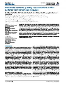
Figure 1: Overview of our model. The imagined representations are the outputs of a text-to-vision mapping.

Introduction

Convolutional neural networks (CNN) and distributionalsemantic models have provided breakthrough advances in representation learning in computer vision (CV) and natural language processing (NLP) respectively (LeCun, Bengio, and Hinton 2015). Lately, a large body of research has shown that using rich, multimodal representations created from combining textual and visual features instead of unimodal representations (a.k.a. embeddings) can improve the performance of semantic tasks. Building multimodal representations has become a popular problem in NLP that has yielded a wide variety of methods (Lazaridou, Pham, and Baroni 2015; Kiela and Bottou 2014; Silberer and Lapata 2014)—a general classification of strategies is proposed in the next section. Additionally, the use of a mapping (e.g., a continuous function) to bridge vision and language has also been explored, typically with the goal of generating missing information from one of the modalities (Lazaridou, Bruni, and Baroni 2014; Socher et al. 2013; Johns and Jones 2012). c 2017, Association for the Advancement of Artificial Copyright Intelligence (www.aaai.org). All rights reserved.

Here, we propose a language-to-vision mapping that provides both a way to “imagine” missing visual information and a method to build multimodal representations. We leverage the fact that by learning to predict the output, the mapping necessarily encodes information from both modalities. Thus, given a word embedding as input, the mapped output is not purely a visual representation but is implicitly associated with the linguistic modality of this word. To the best of our knowledge, the use of mapped vectors to build multimodal representations has not been considered before. Additionally, our method introduces a cognitively plausible approach to concept representation. By re-constructing visual knowledge from textual input, our method behaves similarly as human memory, namely in an associative and re-constructive manner (Anderson and Bower 2014; Vernon 2014; Hawkins and Blakeslee 2007). Concretely, the goal of our method is not the perfect recall of visual representations but rather its re-construction and association with textual knowledge. In contrast to other multimodal approaches such as skipgram methods (Lazaridou, Pham, and Baroni 2015; Hill and

Korhonen 2014) our method of directly learning from pretrained embeddings instead of training from a large multimodal corpus is simpler and faster. Hence, the proposed method can alternatively be seen as a fast and easy way to generate multimodal representations from purely unsupervised linguistic input. Because annotated visual representations are more scarce than large unlabeled text corpora, generating multimodal representations from pre-trained unsupervised input can be a valuable resource. By using seven test sets covering three different similarity tasks (semantic, visual and relatedness), we show that the imagined visual representations help to improve performance over strong unimodal baselines and state-of-the-art multimodal approaches. We also show that the imagined visual representations concatenated to the textual representations outperform the original visual representations concatenated to the same textual representations. The proposed method also performs well in zero-shot settings, hence indicating good generalization capacity. In turn, the fact that our evaluation tests are composed of human ratings of similarity supports our claim that our method provides more human-like judgments. The rest of the paper is organized as follows. In the next section, we introduce related work and background. Then, we describe and provide insight on the proposed method. Afterwards, we describe our experimental setup. Finally, we present and discuss our results, followed by conclusions.

mental search necessarily includes both, the visual and the semantic component. For this reason, we consider the concatenation of the imagined visual representations to the text representations as a powerful way of comprehensively representing concepts.

2.2

Multimodal representations

Psychological research evidences that human concept formation is strongly grounded in visual perception (Barsalou 2008), suggesting that a potential semantic gain can be derived from fusing text and visual features. It has also been empirically shown that distributional semantic models and visual CNN features capture complementary attributes of concepts (Collell and Moens 2016). The combination of both modalities had been considered since a long time ago (Loeff, Alm, and Forsyth 2006), and its advantages have been largely demonstrated in a number of linguistic tasks (Lazaridou, Pham, and Baroni 2015; Kiela and Bottou 2014; Silberer and Lapata 2014). Based on current literature, we present a general classification of the existing approaches. Broadly, we consider two families of strategies: a posteriori combination and simultaneous learning. That is, multimodal representations are built by learning from raw input enriched with both modalities (simultaneous learning) or by learning each modality separately and integrating them afterwards (a posteriori combination). 1. A posteriori combination.

2 2.1

Related work and background

Cognitive grounding

A large body of research evidences that human memory is inherently re-constructive (Vernon 2014; Hawkins and Blakeslee 2007). That is, memories are not exact static copies of reality, but are rather re-constructed from its essential elements each time they are retrieved, triggered by either internal or external stimuli and often modulated by our expectations. Arguably, this mechanism is, in turn, what endows humans with the capacity to imagine themselves in yet-to-be experiences and to re-combine existing knowledge into new plans or structures of knowledge (Hawkins and Blakeslee 2007). Moreover, the associative nature of human memory is also a widely accepted theory in experimental psychology (Anderson and Bower 2014) with identifiable neural correlates involved in both learning and retrieval processes (Reijmers et al. 2007). In this respect, our method employs a retrieval process analogous to that of humans, in which the retrieval of a visual output is triggered and mediated by a linguistic input (Fig. 1). Effectively, visual information is not only retrieved (i.e., mapped), but also associated to the textual information thanks to the learned cross-modal mapping—which can be interpreted as a human mental model of the association between the semantic and visual components of concepts, acquired through lifelong experience. Finally, the retrieved (mapped) visual information is often insufficient to completely describe a concept, and thus it is of interest to preserve the linguistic component. Analogously, when humans face the same similarity task (e.g., “cat” vs. “tiger”) their

• Concatenation. The simplest approach to fuse prelearned visual and text features is by concatenating them (Kiela and Bottou 2014). Variations of this method include the application of single value decomposition (SVD) to the matrix of concatenated visual and textual embeddings (Bruni, Tran, and Baroni 2014). Concatenation has been proven effective in concept similarity tasks (Bruni, Tran, and Baroni 2014; Kiela and Bottou 2014), yet has an obvious limitation: multimodal features can only be generated for those words that have images available, thus reducing the multimodal vocabulary drastically. • Autoencoders form a more elaborated approach that do not suffer from the above problem. Encoders are fed with pre-learned visual and text features, and the hidden representations are then used as multimodal embeddings. This approach has shown to perform well in concept similarity tasks and categorization (i.e., grouping objects into categories such as “fruit”, “furniture”, etc.) (Silberer and Lapata 2014). • A mapping between visual and text modalities (i.e., our method). The outputs of the mapping themselves are used in the multimodal representations. 2. Simultaneous learning. Distributional semantic models are extended into the multimodal domain (Lazaridou, Pham, and Baroni 2015; Hill and Korhonen 2014) by learning in a skip-gram manner from a corpus enriched with information from both modalities and using the learned parameters of the hidden layer as multimodal representation. Multimodal skip-gram methods have been

proven effective in similarity tasks (Lazaridou, Pham, and Baroni 2015; Hill and Korhonen 2014), in zero-shot image labeling (Lazaridou, Pham, and Baroni 2015) and in propagating visual knowledge into abstract words (Hill and Korhonen 2014). With this classification, the gap that our method fills becomes more clear, with it being the most aligned with the re-constructive view of knowledge representation (Vernon 2014; Loftus 1981) that seeks the explicit association between vision and language.

2.3

Cross-modal mappings

Several studies have considered the use of mappings to bridge modalities. For instance, Socher et al. (2013) and Lazaridou, Bruni, and Baroni (2014) use a linear vision-tolanguage projection to perform zero-shot image classification (i.e., classifying images from a class not seen during training). Analogously, language-to-vision mappings have been considered, generally to generate missing perceptual information about abstract words (Hill and Korhonen 2014; Johns and Jones 2012) and in zero-shot image retrieval (Lazaridou, Pham, and Baroni 2015). In contrast to our approach, the methods above do not aim to build multimodal representations to be used in natural language processing tasks.

3

3.2

Learning to map language to vision

Let L ⊂ Rdl be the linguistic space and V ⊂ Rdv the visual space of representations, where dl and dv are the sizes of → − the text and visual representations respectively. Let lw ∈ L and − v→ w ∈ V denote the text and visual representations for the concept w respectively. Our goal is to learn a mapping → − (regression) f : L → V such that the prediction f (lw ) is − → “similar” to the actual visual vector vw . The set of N visual representations (described in the subsection 3.1) along with their corresponding text representations compose the train→ − − N ing data {( li , → vi )}i=1 used to learn the mapping f . In this work, we consider two different mappings f . (1) Linear: A simple perceptron composed of a dl dimensional input layer and a linear output layer with dv units (Fig. 2, left). (2) Neural network: A network composed of a dl -unit input layer, a single hidden layer of dh Tanh units and a linear output layer of dv units (Fig. 2, right).

Proposed method

In this section, we first describe the three main steps of our method (Fig. 1): (1) Obtain visual representations of concepts; (2) Build a mapping from the linguistic to the visual space; and (3) Generate multimodal representations. Afterwards, we provide insight on our approach.

3.1

Obtaining visual representations

We employ raw, labeled images from ImageNet (Russakovsky et al. 2015) as the source of visual information (see section 4), although alternative sources such as the ESP game data set (Von Ahn and Dabbish 2004) or Google image search can be used. We suggest however that both, the number of images per concept and the total number of concepts N should be of a reasonable amount. To extract visual features from each image, we use the forward pass of a pre-trained CNN model. The hidden representation of the last layer (before the softmax) is often taken as a feature vector, as it contains higher level features. Although bags of visual words such as SIFT (Lowe 1999) or HOG (Dalal and Triggs 2005) may also be considered, they generally yield lower performance than CNNs (Kiela and Bottou 2014). For each concept w, we consider two different ways of combining the extracted visual features of individual images into a single representation − v→ w. (1) Averaging: Component-wise average of the feature vectors of the individual images. (2) Maxpooling: Component-wise maximum of all feature vectors of individual images. This can be interpreted as bags of visual properties.

Figure 2: Architecture of the linear (left) and neural network (right) mappings. For both, linear and neural network mappings, a mean squared error (MSE) loss function is employed: 1 ||ˆ y − y||22 2 where y is the actual (multidimensional continuous) output and yˆ the model prediction. The inclusion of cross-modality mappings that are symmetrical with respect to input and output such as canonical correlation analysis (CCA) would deviate from the target of this work, which assumes directionality. However, a comparison with CCA is briefly discussed in the Results section. Loss(y, yˆ) =

3.3

Generating multimodal representations

As a final step, the imagined representation − m→ w of each con→ − cept w is calculated as the image f (lw ) of its linguistic em→ − → − bedding lw —where we notice that the input vector lw has not necessarily been seen at training time. E.g., the imagined

−−→ −−− → representation of w = dog corresponds to m dog = f (ldog ). We henceforth refer to the mapped or imagined representations as MAPf , where f indicates the mapping function employed (lin = linear, N N = neural network). As argued in subsection 3.4, the imagined representations are effec→ − tively multimodal. However, since the predictions f (lw ) formally belong to the visual domain, we also consider the multimodal representations built by concatenating the `2 → − normalized imagined representations f (lw ) with the textual → − → − → − representations lw , namely lw ⊕ f (lw ), where ⊕ denotes the concatenation operator. We henceforth denote these concatenated representations as MAP-Cf , with f indicating the mapping employed.

3.4

Intuition of the method

Since the outputs of a text-to-vision mapping are strictly speaking, visual predictions, it might not be readily obvious that they contain multimodal information. To gain insight on this question, it is instructive to refer to the training phase where the parameters θ of f are learned as a function → − − N of the training data {( li , → vi )}i=1 . For instance, in gradient descent, θ is updated according to ∂ → − − N θ(t+1) = θ(t) − η (t) Loss(θ; {( li , → vi )}i=1 ). ∂θ Hence, the parameters θ of f are effectively a function of → − − N the training data points {( li , → vi )}i=1 involving an explicit dependency on both, input and output data. It is thus ex→ − pected that the outputs f (lw ) are grounded with properties → − N of the input data { li }i=1 . It can be additionally noted that → − the output of the mapping f (lw ) is a (continuous) transfor→ − mation of the input vector lw . Thus, unless the mapping is completely uninformative (e.g., a constant or a random map→ − ping), the input vector lw will still be “present”—yet transformed. In fact, the range of transformations that a linear model can perform to the input space is limited (scaling, reflection, rotation, shearing and translation)—assuming nonsingular θ. Similarly, a neural network with Tanh units preserves the topological properties of the input space, involving thus “stretching” and “squishing” but not cutting. Additionally, by using the visual predictions of a mapping that explicitly associates language to vision we seek to avoid the inclusion of noise from the visual representations into the multimodal ones. During the learning phase, irrelevant visual information and noise are discarded to a large extent, which leads us to hypothesize that the mapped vectors are semantically richer than the original visual vectors.

4 4.1

Experimental setup

Word embeddings

We use 300-dimensional GloVe1 vectors (Pennington, Socher, and Manning 2014) pre-trained on the Common Crawl corpus consisting of 840B tokens and a 2.2M words vocabulary. This embedding choice is motivated by its stateof-the-art performance (Pennington, Socher, and Manning 2014), which provides a strong base to learn the mappings. 1

http://nlp.stanford.edu/projects/glove

4.2

Visual data and features

We use ImageNet (Russakovsky et al. 2015) as our source of visual information. This choice is motivated by: (i) Ease of replicating our experiment, (ii) High quality and low noise of images, and (iii) Large vocabulary coverage. ImageNet covers a total of 21,841 WordNet synsets (or meanings) (Fellbaum 1998) and has 14,197,122 images. For our experiment, we only keep synsets with more than 50 images, and an upper bound of 500 images per synset is used to reduce computation time. With this selection, we cover 9,251 unique words, taken as the most relevant word of each synset. Hence, our training data is composed of N = 9,251 → − → instances or (lw , − vw ) pairs. To extract visual features from each image, we use a pretrained VGG-m-128 CNN model (Chatfield et al. 2014) implemented with the Matlab MatConvNet toolkit (Vedaldi and Lenc 2015). We take the 128-dimensional activation of the last layer (before the softmax) as our visual feature vector − v→ w.

4.3

Evaluation sets

We tested the proposed method with 7 benchmark tests, covering three different tasks: (i) General relatedness: MEN (Bruni, Tran, and Baroni 2014) and Wordsim353-rel (Agirre et al. 2009); (ii) Semantic or taxonomic similarity: SemSim (Silberer and Lapata 2014), Simlex999 (Hill, Reichart, and Korhonen 2015), Wordsim353-sim (Agirre et al. 2009) and SimVerb-3500 (Gerz et al. 2016); (iii) Visual similarity: VisSim (Silberer and Lapata 2014) which contains the same word pairs as SemSim, rated for visual similarity instead of semantic similarity. All test sets contain pairs of words along with their associated human similarity rating. The tests Wordsim353-sim and Wordsim353-rel correspond to the similarity and relatedness subsets of the original Wordsim353 (Finkelstein et al. 2001) respectively, as proposed by Agirre et al. (2009) who noted that the distinction between similarity (e.g., “tiger” is similar to “cat”) and relatedness (e.g., “stock” is related to “market”) yields different results. Hence, for being redundant with its subsets, we do not count the whole Wordsim353 as an extra test set, yet it is included in the Results section for completeness. It is important to notice that a large part of words in our test sets do not have a visual representation − v→ w available, i.e., they are not present in our training data. We refer to these words as zero-shot (ZS).

4.4

Evaluation metric and prediction

We employ Spearman correlation ρ between model predictions and human similarity ratings as evaluation metric. The prediction of similarity between two concept representa→1 and − →2 , is computed by their cosine similarity: tions, − u u − → − → →1 , − →2 ) = u1 · u2 cos(− u u − →1 k · ku − →2 k ku

4.5

Model settings

Both, neural network and linear models are learned by stochastic gradient descent and a total of nine parameter

combinations are tested (learning rate = [0.1, 0.01, 0.005] and dropout rate = [0.5, 0.25, 0.1]). We find that the models are not very sensitive to variations (especially of the dropout rate) and all of them perform reasonably well. We report a linear model with learning rate of 0.1 and dropout rate of 0.1, running it for 175 epochs. For the neural network, we additionally test three different architectures with 50, 150 and 300 hidden units. We find performance with 150 and 300 hidden units to be almost identical, whilst performance with 50 units slightly drops. We report a neural network with 300 hidden units, dropout rate of 0.25 and learning rate of 0.1, trained for 25 epochs. All mappings are implemented with the scikit-learn toolkit (Pedregosa et al. 2011) and our embeddings are publicly available2 .

5

Results and discussion

For clarity, the following notation is introduced. We refer to the averaged and maxpooled visual features as CNN avg and CNN max respectively. CONC refers to the concatenation of CNN avg and GloVe, which can be seen as the same method of Kiela and Bottou (2014) with our base unimodal representations. Since maxpooled and averaged visual representations performed similarly (both, the CNN features and the mappings learned from them), only results on averaged representations are discussed below and in Tab. 1. Overall performance We perform post-hoc Nemenyi tests by regarding the disjoint regions of each test set (i.e., ZS and VIS) as different sets, which yields 14 sets (excluding Worsim353). We find that both MAP-Clin and MAPCN N perform significantly better than GloVe (p ≈ 0.03) and than CNN avg (p ≈ 0.06)—the latter test includes only the seven VIS regions. Therefore, our multimodal representations MAP-C clearly accomplish one of their foremost goals, namely to improve the unimodal representations of GloVe and CNN avg . Multimodal grounding Clearly, the consistent improvement of MAPlin and MAPN N over CNN avg in all seven test sets supports our claim that the imagined visual representations are more than purely visual representations and contain multimodal information—as analytically argued in subsection 3.4. Moreover, the MAP-C method generally performs better than the MAP vectors alone, implying that even though the MAP vectors are indeed multimodal, they are still predominantly visual and therefore their concatenation with textual representations helps. Concreteness By employing the concreteness ratings of Brysbaert, Warriner, and Kuperman (2014) in a 1-5 scale (with 5 being the most concrete and 1 the most abstract) we find that the average concreteness in the VIS regions is 4.6± 0.5, which is substantially larger than the average of 3.2±0.9 in the ZS regions. Importantly, the average concreteness is larger than 4.4 in all VIS regions, while it is lower than 3.3 in all ZS regions except in MEN and VisSim/SemSim test sets which average 4.2 and 4.8 respectively. Therefore, with 2

http://liir.cs.kuleuven.be/software.php

Figure 3: Sample of images from the “car” (top row) and “garage” (bottom row) synsets of ImageNet. the exceptions of MEN, VisSim and SemSim, the inclusion of multimodal information in the ZS regions can be generally regarded as less beneficial than in the VIS regions, given that visual information can only sensibly enrich representations of words that are to some extent visual. Visual (VIS) regions Crucially, MAP-CN N and MAPClin significantly improve the performance of GloVe in all seven VIS regions (p ≈ 0.008), with an average improvement of 4.6% for MAP-CN N and 2.8% for MAP-Clin . Conversely, the concatenation of GloVe with the original visual vectors (CONC) does not improve GloVe (p ≈ 0.7)— worsening it in 4 out of 7 test sets—suggesting that simple concatenation without seeking the association between modalities might be suboptimal. Moreover, the concatenation of the imagined visual vectors with GloVe (MAP-CN N ) outperforms the concatenation of the original visual vectors with GloVe (CONC) in 6 out of 7 test sets (p ≈ 0.06), which supports our claim that the imagined visual vectors are semantically richer and less noisy than the original visual vectors. Zero-shot (ZS) regions Given the above considerations on concreteness, as expected, MAP-C methods substantially improve GloVe performance in the ZS regions of VisSim and SemSim, and more slightly in MEN. Interestingly, MAP-C also improves GloVe in the ZS region of SimVerb-3500, yet only marginally. General relatedness Both MAPN N and MAPlin exhibit an overall gain in MEN and in the VIS region of Wordsim353-rel. It might seem perhaps counter-intuitive that vision can help to improve relatedness understanding. However, a closer look to the particular examples reveals that visual features generally account for object cooccurrences, which is often a good indicator of their relatedness. For instance, in MEN, the human relatedness rating between “car” and “garage” is 8.2 while GloVe’s score is only 5.4. However, CNN avg ’s rating is 8.7 and that of MAPnn is 8.4, which is closer to the human score. From Fig. 3, the co-occurrences of garage-car is clear. Visual similarity MAPN N attains the best performance in VisSim, especially in the ZS subset. Regardless, both MAPClin and MAP-CN N outperform the two unimodal baselines.

Silberer & Lapata 2014 Lazaridou et al. 2015 Kiela & Bottou 2014 GloVe CNN avg CONC MAPN N MAPlin MAP-CN N MAP-Clin # inst.

ALL 0.712 0.443 0.402 0.687 0.694 353

Wordsim353 VIS ZS 0.61 0.632 0.705 0.448 0.606 0.534 0.391 0.539 0.366 0.644 0.673 0.649 0.684 63 290

GloVe CNN avg CONC MAPN N MAPlin MAP-CN N MAP-Clin # inst.

ALL 0.75 0.805 0.703 0.701 0.813 0.811 3000

MEN VIS 0.76 0.72 0.801 0.593 0.8 0.761 0.774 0.82 0.819 795

ZS 0.801 0.68 0.674 0.806 0.802 2205

Wordsim353-rel ALL VIS ZS 0.644 0.759 0.619 0.422 0.665 0.33 0.606 0.267 0.28 0.553 0.243 0.623 0.778 0.589 0.629 0.797 0.601 252 28 224

ALL 0.7 0.72 0.753 0.729 0.738 0.783 0.785 6933

SemSim VIS 0.72 0.768 0.534 0.734 0.732 0.738 0.791 0.791 5238

ZS 0.701 0.718 0.74 0.754 0.764 1695

Wordsim353-sim ALL VIS ZS 0.802 0.688 0.783 0.526 0.664 0.536 0.599 0.475 0.505 0.569 0.477 0.769 0.696 0.745 0.781 0.698 0.766 203 45 158

ALL 0.64 0.63 0.591 0.658 0.646 0.65 0.641 6933

VisSim VIS 0.63 0.606 0.56 0.651 0.659 0.644 0.657 0.647 5238

ZS 0.54 0.655 0.651 0.626 0.623 1695

ALL 0.4 0.408 0.322 0.322 0.405 0.41 999

Simlex999 VIS ZS 0.53 0.371 0.429 0.406 0.442 0.451 0.296 0.412 0.286 0.404 0.417 0.388 0.422 261 738

SimVerb-3500 ALL VIS ZS 0.283 0.32 0.282 0.235 0.437 0.213 0.513 0.21 0.212 0.338 0.21 0.286 0.49 0.284 0.286 0.371 0.285 3500 41 3459

Table 1: Spearman correlations between model predictions and human ratings. For each test, ALL correspond to the whole set of word pairs, VIS to those pairs for which we have both visual representations, and ZS denotes its complement, i.e., zero-shot words. Boldface indicates the best results per column and # inst. the number of word pairs in each region (ALL, VIS, ZS). We notice that comparison methods are not available for test sets in the second row. Additionally, the VIS subset of the compared methods is only approximated, as the authors do not report the exact evaluated instances. Unimodal baselines We use low dimensional (128-d) visual representations to reduce the number of parameters— and thus the risk of overfitting. However, to test whether results are independent of the choice of the CNN, we repeat the experiment using a pre-trained AlexNet CNN model (Krizhevsky, Sutskever, and Hinton 2012) (4096dimensional features) and a ResNet CNN (He et al. 2015) (2048-dimensional features) and find that both perform similar to the VGG-m-128 CNN reported here. Not only the visual representations (CNN avg ) perform closely, but the mapped vectors perform similarly too. On the linguistic side, we additionally test word2vec (Mikolov et al. 2013) word embeddings, which fare marginally worse than GloVe—both, the text embeddings themselves and the imagined vectors learned from them. Thus, we report results on our strongest text baseline. Mappings MAP-CN N and MAP-Clin exhibit similar performance trends. However, MAP-CN N generally shows larger improvements in the VIS regions with respect to GloVe than MAP-Clin does, arguably because the neural network is able to better fit the visual vectors, thus preserving more information from the visual modality. In fact, it can be observed that the performance of MAP-CN N generally deviates more from that of GloVe than MAP-Clin does. We additionally find (not shown in Tab. 1) that MAPlin from a linear model trained for only 2 epochs improves GloVe in 5 of our test sets, with an average improvement of ≈ 3%. However, the R2 fit of this model is lower than 0 and thus we cannot guarantee that the improvement comes from the visual vectors. We attribute this gain to an artifact caused by scaling and smoothing effects of backpropagation, yet more research is needed to better understand this effect.

For completeness, we test a CCA model learned in our training data as a baseline method (not shown here). It consistently performs worse than GloVe in each test, suggesting that mapping into a common latent space might not be an appropriate solution to the problem at hand.

6

Conclusions

We have presented a cognitively-inspired method capable of generating multimodal representations in a fast and simple way by using pre-trained unimodal text and visual representations as a starting point. In a variety of similarity tasks and 7 benchmark tests, our method generally outperforms strong unimodal baselines and state-of-the-art multimodal methods. Moreover, the proposed method exhibits good performance in zero-shot settings, indicating that the model generalizes well and learns relevant cross-modal associations. In conclusion, its effectiveness as a simple method to generate multimodal representations from purely unsupervised linguistic input is supported. Finally, the overall performance increase supports the claim that our approach builds more human-like concept representations. Ultimately, the present paper sheds light on fundamental questions of natural language understanding such as the plausibility of re-constructive and associative processes to fuse vision and language. The present work advocates for more cognitively inspired methods, although we aim to inspire researchers to further investigate this question.

Acknowledgments This work has been supported by the CHIST-ERA EU project MUSTER3 . We additionally thank our anonymous reviewers for the helpful comments.

References Agirre, E.; Alfonseca, E.; Hall, K.; Kravalova, J.; Pas¸ca, M.; and Soroa, A. 2009. A study on similarity and relatedness using distributional and wordnet-based approaches. In NAACL, 19–27. ACL. Anderson, J. R., and Bower, G. H. 2014. Human Associative Memory. Psychology press. Barsalou, L. W. 2008. Grounded cognition. Annu. Rev. Psychol. 59:617–645. Bruni, E.; Tran, N.-K.; and Baroni, M. 2014. Multimodal distributional semantics. JAIR 49(1-47). Brysbaert, M.; Warriner, A. B.; and Kuperman, V. 2014. Concreteness ratings for 40 thousand generally known english word lemmas. Behavior research methods 46(3):904– 911. Chatfield, K.; Simonyan, K.; Vedaldi, A.; and Zisserman, A. 2014. Return of the devil in the details: Delving deep into convolutional nets. In BMVC. Collell, G., and Moens, S. 2016. Is an image worth more than a thousand words? on the fine-grain semantic differences between visual and linguistic representations. In COLING. ACL. Dalal, N., and Triggs, B. 2005. Histograms of oriented gradients for human detection. In CVPR, volume 1, 886–893. IEEE. Fellbaum, C. 1998. WordNet. Wiley Online Library. Finkelstein, L.; Gabrilovich, E.; Matias, Y.; Rivlin, E.; Solan, Z.; Wolfman, G.; and Ruppin, E. 2001. Placing search in context: The concept revisited. In WWW, 406–414. ACM. Gerz, D.; Vuli´c, I.; Hill, F.; Reichart, R.; and Korhonen, A. 2016. Simverb-3500: A large-scale evaluation set of verb similarity. arXiv preprint arXiv:1608.00869. Hawkins, J., and Blakeslee, S. 2007. On Intelligence. Macmillan. He, K.; Zhang, X.; Ren, S.; and Sun, J. 2015. Deep residual learning for image recognition. arXiv preprint arXiv:1512.03385. Hill, F., and Korhonen, A. 2014. Learning abstract concept embeddings from multi-modal data: Since you probably can’t see what i mean. In EMNLP, 255–265. Hill, F.; Reichart, R.; and Korhonen, A. 2015. Simlex-999: Evaluating semantic models with (genuine) similarity estimation. Computational Linguistics 41(4):665–695. Johns, B. T., and Jones, M. N. 2012. Perceptual inference through global lexical similarity. Topics in Cognitive Science 4(1):103–120. 3

http://www.chistera.eu/projects/muster

Kiela, D., and Bottou, L. 2014. Learning image embeddings using convolutional neural networks for improved multimodal semantics. In EMNLP, 36–45. Citeseer. Krizhevsky, A.; Sutskever, I.; and Hinton, G. E. 2012. Imagenet classification with deep convolutional neural networks. In NIPS, 1097–1105. Lazaridou, A.; Bruni, E.; and Baroni, M. 2014. Is this a wampimuk? cross-modal mapping between distributional semantics and the visual world. In ACL, 1403–1414. Lazaridou, A.; Pham, N. T.; and Baroni, M. 2015. Combining language and vision with a multimodal skip-gram model. arXiv preprint arXiv:1501.02598. LeCun, Y.; Bengio, Y.; and Hinton, G. 2015. Deep learning. Nature 521(7553):436–444. Loeff, N.; Alm, C. O.; and Forsyth, D. A. 2006. Discriminating image senses by clustering with multimodal features. In COLING/ACL, 547–554. ACL. Loftus, E. F. 1981. Reconstructive memory processes in eyewitness testimony. In The Trial Process. Springer. 115– 144. Lowe, D. G. 1999. Object recognition from local scaleinvariant features. In CVPR, volume 2, 1150–1157. IEEE. Mikolov, T.; Sutskever, I.; Chen, K.; Corrado, G. S.; and Dean, J. 2013. Distributed representations of words and phrases and their compositionality. In NIPS, 3111–3119. Pedregosa, F.; Varoquaux, G.; Gramfort, A.; Michel, V.; Thirion, B.; Grisel, O.; Blondel, M.; Prettenhofer, P.; Weiss, R.; Dubourg, V.; Vanderplas, J.; Passos, A.; Cournapeau, D.; Brucher, M.; Perrot, M.; and Duchesnay, E. 2011. Scikitlearn: Machine learning in Python. JMLR 12:2825–2830. Pennington, J.; Socher, R.; and Manning, C. D. 2014. Glove: Global vectors for word representation. In EMNLP, volume 14, 1532–1543. Reijmers, L. G.; Perkins, B. L.; Matsuo, N.; and Mayford, M. 2007. Localization of a stable neural correlate of associative memory. Science 317(5842):1230–1233. Russakovsky, O.; Deng, J.; Su, H.; Krause, J.; Satheesh, S.; Ma, S.; Huang, Z.; Karpathy, A.; Khosla, A.; Bernstein, M.; et al. 2015. Imagenet large scale visual recognition challenge. IJCV 115(3):211–252. Silberer, C., and Lapata, M. 2014. Learning grounded meaning representations with autoencoders. In ACL, 721–732. Socher, R.; Ganjoo, M.; Manning, C. D.; and Ng, A. 2013. Zero-shot learning through cross-modal transfer. In NIPS, 935–943. Vedaldi, A., and Lenc, K. 2015. Matconvnet – convolutional neural networks for matlab. In Proceeding of the ACM Int. Conf. on Multimedia. Vernon, D. 2014. Artificial Cognitive Systems: A primer. MIT Press. Von Ahn, L., and Dabbish, L. 2004. Labeling images with a computer game. In SIGCHI conference on Human factors in computing systems, 319–326. ACM.