Specifically, we are interested in a particular class of closed loop curves in 2D with multiple self-crossings which bound a surface homeomorphic to a ... The top left figure is an input to our algorithm. ... plane such that we can see only the blue side of the disk. .... longing to cells with winding number 1 and joining them by.
EUROGRAPHICS Symposium on Sketch-Based Interfaces and Modeling (2011) T. Hammond and A. Nealen (Editors)
Immersion and Embedding of Self-Crossing Loops Uddipan Mukherjee1 , M.Gopi1 , and Jarek Rossignac2 1 University 2 Georgia
of California, Irvine, USA Institute of Technology, USA
Abstract The process of generating a 3D model from a set of 2D planar curves is complex due to the existence of many solutions. In this paper we consider a self-intersecting planar closed loop curve, and determine the 3D layered surface P with the curve as its boundary. Specifically, we are interested in a particular class of closed loop curves in 2D with multiple self-crossings which bound a surface homeomorphic to a topological disk. Given such a selfcrossing closed loop curve in 2D, we find the deformation of the topological disk whose boundary is the given loop. Further, we find the surface in 3D whose orthographic projection is the computed deformed disk, thus assigning 3D coordinates for the points in the self-crossing loop and its interior space. We also make theoretical observations as to when, given a topological disk in 2D, the computed 3D surface will self-intersect.
1. Introduction Given the sketch of a 2D planar curve, the problem of finding the 3D space curve and the surface bounded by it is mathematically indeterminable, as it has many possible solutions. It is well known that the basic difficulty is in choosing the appropriate one. Many sketch-based modeling systems try to avoid addressing this fundamental problem directly due to its complexity. These systems provide a fixed canvas to the user to draw the 2D curve, thus fixing the 3D curve to be on the canvas. They provide tools to change the shape of the canvas to enable the user to draw non-planar curves [IITS, IMT99]. All of these approaches first generate nonplanar 3D curves from the planar 2D curves, which then become the fundamental component of 3D surface generation [ZHH96,IH03]. Another approach in reconstructing 3D models from 2D sketches is to use priors based on geometric properties like parallelism and perpendicularity of edges [LS96]. In this approach, the 2D graph drawn by the user is elevated to 3D using these priors. Other types of priors used to obain a 3D model from a single 2D sketch are visible contours of the model or cusps and T-junctions [KH06]. Learning approach is also sometimes incorporated to make use of correlations between different 3D objects [LS00, SC04]. Recent research on surface generation also use implicit surface representation techniques like creating convolution surface from sketched silhouettes [lTZkF04], or subdivision surfaces from curve network [SWZ04]. c The Eurographics Association 2011.
Figure 1: Obtaining a 3D layered surface from a closedloop curve. The top left figure is an input to our algorithm. All the other figures show the generated 3D layered surface from different viewpoints, such that when this surface is projected onto an underlying 2D plane, its boundary is the input 2D closed-loop curve.
In spite of all the successes that have been achieved in the field of sketch based modeling, the fundamental problem of space curve determination still remains to be a challenging one. A mathematically sound insight to this problem is provided in [DDgG05]. Given an open self-crossing 2D curve with known 3D coordinates of its end points, [DDgG05] finds a curvature minimizing 3D curve whose orthographic projection is the given 2D curve. In our paper, given a closed self-crossing 2D loop curve, we find a surface patch in 3D, the orthographic projection of whose boundary is the given 2D curve. Figure 1 shows an example.
Uddipan Mukherjee & M.Gopi & Jarek Rossignac / Immersion and Embedding of Self-Crossing Loops
1.1. Problem Statement In this paper we are only concerned about planar closedloop curves which may intersect itself multiple times. We call this class of curves self-crossing loops. The concept of self-crossing loops is explained nicely in [SVW92]. Suppose we paint a planar disk red on one side and blue on the other side and set our viewing direction perpendicular to the plane such that we can see only the blue side of the disk. If we deform the disk without lifting it off the plane then the deformed disk may self intersect many times but we will still see only its blue side. The boundary of this deformed disk forms a self-crossing loop which, we say, is immersible. We call the deformation pattern of the disk in 2D as an immersion. However, if during the process of deforming the disk, we lift it at any time and give it one or more twists, we will be able to see both the colors. In this case, the boundary of the twisted disk is still a self-crossing loop but we call it nonimmersible. Figure 2 illustrates these concepts.
possible immersions, in which two different triangulations of same immersion are considered as two unique solutions. Using this algorithm, the worst case time complexity of finding both one and all immersions is O(n3 ) where n is the number of vertices on the self-crossing loop. On the other hand, we present an algorithm with worst case complexity of O(k) to compute one immersion, where k is the number of crossing points, and O(k2 ) to compute all immersions. Although polygons can be designed where k can be up to n2 , in all practical cases, k is much less than n. For example, in Figure 4, number of vertices, n of the polygon is 16, while the number of crossing points, k is 8. Hence our algorithm to find an immersion from a self-crossing loop is much faster and more suitable for interactive sketch based modeling applications than the only existing solution for this problem. Further, to the best of our knowledge we present the first algorithm to assign layers to the immersion to lift the selfcrossing loop into a non self intersecting 3D surface patch called an embedding. We also present many other theoretical results that improves the current understanding to answer many open questions related to this problem. 1.2. Main Contributions Following are the main contributions of our paper:
Figure 2: Immersible and non-immersible self-crossing loops. A planar disk is painted blue (visible) on one side and red (not visible) on the other. Top: The disk is deformed to form an immersible self-crossing loop. Observe that we can see only the blue color. Bottom: the disk is twisted to form a non-immersible loop. Here we can see both the colors of the disk. The boundaries of the disk form self-crossing loops in each case. The problem of finding an immersion from a self-crossing loop is complicated due to the fact that there may exist many immersions corresponding to the loop. Figure 3 shows an example of a self-crossing loop with two immersions.
• Given a self-crossing loop, we determine whether it is immersible in worst case complexity of O(n2 ), which was posed as an open question in [SVW92]. • If the self-crossing loop is immersible, we apply a novel algorithm, which runs in time linear in the number of crossing points of the loop, to compute an immersion. • We lift this 2D immersion to 3D such that self-intersection in the 3D surface is avoided, if possible. If the 3D surface does not self-intersect, it is called an embedding. Figure 4 shows the formation of immersion of a self-crossing loop and the corresponding embedding. The progress of the shaded region in the sequence of figures traces out a locus of the deformation pattern of the disk. • The complexity class of the problem of taking a selfcrossing loop directly to an embedding (instead of first finding an immersion and then lifting it to an embedding) is still open [EM09]. As theoretical contribution to this problem, we observe certain sufficiency conditions on embedding an immersion, that may be useful in answering this important open problem.
Figure 3: Left: A self-crossing loop, Center and Right: Two different immersions of the loop. The different sections of the immersion are illustrated with different colors in each case. Our goal is to find an immersion, if one exists, from a selfcrossing loop, and lift it to 3D, avoiding self-intersection of the 3D surface if possible.
Figure 4: Left: The four figures show how a disk has been deformed to form an immersion, Right: Corresponding embedding.
Given a self-crossing loop, [SVW92] can compute all c 2011 The Author(s)
c 2011 The Eurographics Association and Blackwell Publishing Ltd. Journal compilation
Uddipan Mukherjee & M.Gopi & Jarek Rossignac / Immersion and Embedding of Self-Crossing Loops
2. Immersion of Self-Crossing Loops In this section we will describe in detail our algorithm for computing an immersion from a self-crossing loop, if there exists one. For a formal definition of the terms immersion and embedding we refer the reader to [EM09]. 2.1. Definitions The self-crossing loop may be represented as a sequence of edge-connected vertices along the curve, where the first and the last vertices are also connected with an edge. We assume that the vertices in the self-crossing loop are in general position, i.e. no three consecutive vertices lie on a straight line and two non-adjacent edges either do not intersect or they intersect at their relative interiors. We define the intersection points of the edges as crossing points. We define a border to be a connected subset of the vertices of the loop between any two successive crossing points. Observe that the selfcrossing loop divides the space into regions such that there is no vertex of the loop in the interior of any of the regions. We refer to these regions as cells. In other words, the cells are the connected components of the complement of the loop in R2 . The winding number of a cell is an integer denoting the total number of times the directed self-crossing loop goes around the cell. Without loss of generality, we assume that if we start traversing the loop from any arbitrary vertex, the interior of the deformed disk will always be on our right. This allows us to associate a border with the cell lying to its right. Figure 5 illustrates these facts.
Figure 5: A self-crossing loop and its crossing points marked with red dots. The number in each cell denote the winding number of that cell. The borders of the loop are colored with different colors. The 1-winding number cells are colored gray, and the 2-winding number cell is colored pink. The regions not enclosed by the loop have winding number 0. If we start traversing the loop from an arbitrary vertex in the direction shown, each border is associated with the cell lying to its right, e.g. the black border is associated with the winding number 1 region lying to its right.
2.2. Disk Layout As we have seen in Section 1.1, an immersion is a deformed topological disk. So, there exists a local homeomorphism between the disk and an immersion. This homeomorphism or one-to-one and onto mapping becomes clear if the deformed c 2011 The Author(s)
c 2011 The Eurographics Association and Blackwell Publishing Ltd. Journal compilation
disk is unwound to bring back to its original circular shape, which we call the disk layout. This is shown in Figure 6. We would like to make the following observations using this illustration. • The boundary of the disk layout is represented by the ordered sequence of borders of the loop. • The number of instances of a cell is same as its winding number. We call each such instance, a face. In Figure 6, a cell B with winding number two appears two times, as B1 and B2 in the immersion, i.e. it has two faces. Each face maps to a distinct non-intersecting region of the disk layout. • Each border appears in exactly one cell, and in exactly one face of that cell, e.g. the blue border in Figure 6 appears in cell B and face B2 . • No two adjacent borders of a cell appear in the same face. • The segmentation of the disk layout defines a pattern by which different faces can be glued along their lines of separation to obtain an immersion (Figure 6).
Figure 6: Top: Immersion unwound to disk layout. Bottom left: Arcs joining borders of same face. These arcs do not intersect each other. Bottom right: The different faces of the loop that can be glued to form an immersion. Note that the faces map to distinct non-intersecting segments in the disk layout. With these observations, the goal is to find the structure of each face of every cell in the gluing pattern. In other words, for each face of every cell, we need to find the borders that appear in it. Once we know which borders appear together in the same face, these faces can be glued to appropriate faces of the adjacent cells in the correct order to obtain an immersion. As observed in Figure 6, if we start with an unpartitioned disk layout and join the borders belonging to same faces by arcs, those arcs never intersect one another and hence the faces divide the disk layout into partitions. This partitioning of the disk establishes local homeomorphism between the disk and the regions enclosed by the given self-crossing loop, thus yielding an immersion.
Uddipan Mukherjee & M.Gopi & Jarek Rossignac / Immersion and Embedding of Self-Crossing Loops
2.3. Immersion Algorithm We present a simple yet powerful recursive algorithm to find an immersion from a self-crossing loop. Our algorithm finds the topology of each face of a cell by systematically finding the group of borders that define a face, and then by gluing these faces to form an immersion. We begin the process by finding the groups of borders belonging to cells with winding number 1 and joining them by arcs in the disk layout. These cells have one face each. Hence this grouping is obvious and the corresponding borders are connected by arcs in the disk layout, in order. If a cell has only one border, that border is marked by a self-arc in the disk layout. In the example of Figure 6, the black and green borders appear alone in their respective cells and hence they are marked by self-arcs in the disk layout, whereas the red and dark blue borders belong to the same 1-winding number cell and hence they are connected by an arc. Each arc partitions the disk. Within each partition the borders are recursively processed, from those belonging to lower to higher winding number cells, ensuring at each step that a newly drawn arc does not intersect any previously drawn arcs or join any two adjacent borders of a cell, thereby maintaining a homeomorphic mapping between the disk and the immersion. Each such arc is called a valid construction. We note that there will always be a 1-winding number cell to start the process since we assume that all the input edges are in general positions. The pseudo code of our algorithm is given in Algorithm 1. We begin by constructing three separate circular linked lists - the c:list consisting of all the borders in the self-crossing loop in the order of their appearance in the loop starting from an arbitrary crossing point, the w:list consisting of all the borders belonging to 1-winding number cells in the same order as they appear in the c:list, followed by all those belonging to the 2-winding number cells in order and so on, and the f:list containing the borders in each cell in the same order as they appear in the c:list. Algorithm 1 DETERMINE IMMERSION Construct c:list, f:list, and w:list while (there exists a border in w:list which is not processed) do PROCESS(head[w:list]) end while if (number of border groups in a cell)>(winding number of the cell) then ERROR → input not a disk end if Figure 7 illustrates how our algorithm works with an example. In this example, we start with the head of the w : list, i.e. border number 0. Since it is the only border in its cell it cannot be grouped with any other border. Next, we move on to border number 4 and group it with border number
Algorithm 2 PROCESS(M) F = next[M] in f:list, C = next[M] in c:list, W = next[M] in w:list if (F==M) then REMOVE M from all 3 lists else if M,F is a valid construction then RECURSE (M,F) REMOVE M from all 3 lists else N=next[F] in f:list while F,N is a valid construction do RECURSE(F,N) REMOVE F from all 3 lists F=N, N=next[N] in f:list end while REMOVE F from all 3 lists PROCESS M end if Algorithm 3 RECURSE(M,F) C = next[M] in c:list, W = next[M] in w:list if ((F==C) AND (F==W)) then Make (M,F) a valid construction REMOVE M from all 3 lists else if N = next[M] in w:list then PROCESS (next[M] in w:list) RECURSE(M,F) else PROCESS (next[M] in c:list) RECURSE(M,F) end if end if
12, since they are not adjacent in their cell. Once they are grouped, we process all the borders lying between them (i.e. borders numbered 5-11) and come up with another arc joining borders numbered 6 and 10. In a similar way, the rest of the disk layout is processed, each time finding an arc not intersecting any previously drawn arc, and recursively processing all the borders lying between them. Each valid construction divides the disk layout and hence the given loop into two parts – each of which is a selfcrossing loop. By recursively processing each of these new loops (and their corresponding partitions in the disk), we can ensure that the local homeomorphism between the region enclosed by the self crossing loop and the corresponding disk partition is maintained and thus we get a valid immersion. The overall time complexity of our immersion finding algorithm is linear in the number of borders of the selfcrossing loop. At each recursive stage of our algorithm if we use an exhaustive search to come up with all possible valid constructions, we can obtain all the possible immersions, if c 2011 The Author(s)
c 2011 The Eurographics Association and Blackwell Publishing Ltd. Journal compilation
Uddipan Mukherjee & M.Gopi & Jarek Rossignac / Immersion and Embedding of Self-Crossing Loops
Figure 7: Top: A self-crossing loop with its borders numbered and shown in different colors. The c : list, w : list and the f : list are also shown. Bottom:different stages of the disk layout as higher and higher winding number borders are grouped (borders which are grouped alone are shown by small self-loop arcs), and the final segmentation of the disk layout.
there exists more than one, in time quadratic in the number of borders. As a pre-processing step, we compute all the self-crossing points of the loop and the winding number of each cell. Our algorithm does not involve any geometric computation except at this preprocessing stage. We use the topological properties of the structure of immersible self-crossing loops to find an immersion. Hence our algorithm is extremely robust against perturbations of vertices in the loop. In contrast the algorithm presented in [SVW92] is purely geometric, uses all the vertices of the loop at all stages of computation, and has an average run time of O(n3 ) with respect to the number of vertices as against our worst case time of O(n2 ).
is not immersible. These invariances are checked in our system to remove those self-crossing loops that are nonimmersible (Figure 9).
Figure 8: Left: a non-immersible loop. The sum of winding numbers of the diagonal cells around the crossing point is 1+1=2 and 0+0=0, which are not equal. Right: an immersible loop wherein the sum of winding numbers of diagonal cells around each self-crossing is 1+1=2 and 2+0=2.
2.4. Non-Immersible Loops For a self-crossing loop we can make the following observations (Figure 8): • The difference in winding number of two adjacent cells is always 1. This follows directly from the consideration that the borders are in general positions, i.e. they do not overlap. • The difference in winding numbers of cells lying diagonally opposite to each other with respect to a crossing point is 0 or 2. Also, if the loop is immersible, the sum of winding numbers of the diagonal cells around a crossingpoint is the same. We have also observed that any twist in the self-crossing loop would violate some of the above invariances, and hence c 2011 The Author(s)
c 2011 The Eurographics Association and Blackwell Publishing Ltd. Journal compilation
Figure 9: Non-immersible loops input to our algorithm produces an error displayed in the form of a small red cross
3. Embedding from Immersion Once we obtain an immersion, we assign 3D coordinates to the self-crossing loop to form a 3D layered surface. If this surface is non-self-intersecting, it defines an embedding. However, the problem of finding an embedding from an immersion is NP complete [EM09]. Hence we are not always
Uddipan Mukherjee & M.Gopi & Jarek Rossignac / Immersion and Embedding of Self-Crossing Loops
guaranteed to obtain an embedding from an immersion in polynomial time. We make a few important observations as to when such an operation is possible in polynomial time. On the other hand, the computational complexity of finding an embedding directly from the self-crossing loop (not through an immersion) is still unknown. Our observations may be used to solve this important open problem. 3.1. Edge-collapsed graph For each cell in the immersion a simplified layout is obtained by collapsing the arcs (valid constructions) in the disk layout corresponding to that cell. We call this an edge collapsed graph. Note that the borders which are not part of any drawn arcs in the disk layout appear in this edge-collapsed graph as individual nodes. Figure 10 shows the process of obtaining such a graph from the disk layout and some examples of edge-collapsed graphs. If the edge-collpased graph for each cell has a linear spanning subtree, then an embedding can be obtained from the immersion.
layers). Each edge joining two nodes in Figure 11 represents the deformation pattern of the part of the disk between the two faces of the same cell representing those two nodes. Hence, this part of the disk must have a height monotonically increasing or decreasing between the two faces of the cell concerned. Thus, in Figure 11(left) if b lies between a and c, no part of the loop intersects itself, which is necessary for an embedding. This can be extended to a linear graph with any number of nodes and a consistent monotonic layering for all cells is guaranteed to produce an embedding. But if b does not lie between a and c, there is a chance that the disk intersects itself at some point. So given a disk layout of the self-crossing loop, we cannot say for sure whether it produces an embedding if b does not lie between a and c. This leads us to the following lemma. Lemma: A linear spanning subtree in an edge-collapsed graph for every cell is sufficient to produce an embeddable solution. Now suppose we have an edge collapsed graph which does not have a linear spanning subtree. The simplest form is shown in Figure 11(right) with layer numbers corresponding to each node. From the above analysis we can say that any linear subgraph of the edge collapsed graph must be monotonically layered to guarantee an embedding. In Figure 11(right) we have 3 linear sub-graphs with layers a − b − c, a − b − d and c − b − d, each of which must be monotonically layered. So, in order to obtain a guaranteed embedding the following three constraints have to be satisfied:
Figure 10: Top: obtaining an edge-collapsed graph of a cell from the circular layout. Bottom: examples of edgecollapsed graphs - the left one does not have a linear spanning subtree and hence cannot produce an embedding, whereas the other two can. As an example, let us consider a simple edge collapsed graph with 3 nodes as shown in Figure 11(left).
Figure 11: Edge-collapsed graph for two different cells. The nodes in each graph represent distinct faces of the cell. The labels for the nodes with assigned integer values represent the layer number of the face. The graph on the left is linear with three nodes and guarantees an embedding, whereas the graph on the right does not have a linear spanning subtree and does not guarantee an embedding Each node in Figure 11(left) represents a face of the cell concerned. Let the 3D height or layer of the faces be named a, b and c as shown (without loss of generality let us assume that a, b, c are integers and that the faces have fixed
1. b lies between a and c, i.e. a > b > c or a < b < c 2. b lies between a and d, i.e. a > b > d or a < b < d 3. b lies between c and d, i.e. c > b > d or c < b < d However, the above three constraints can never be satisfied simultaneously. e.g. if a > b > c, then a > b > d, and from constraint 3 above, we get c > b > d which is a contradiction. So, if the spanning subtree of the edge-collapsed graph is not linear, an embedding is not guaranteed. Figure 12 shows two examples which produce an embeddable solution, and an example which may or may not produce an embeddable solution depending on the nature of the edge collapsed graph. 3.2. Summary of Observations An edge-collapsed graph with a linear or 2-constrained spanning subtree is sufficient to produce an embedding. The problem of finding whether a k-constrained spanning subtree exists in a graph is NP complete and hence the problem of finding an embedding from an immersion, which is an instance of finding a 2-constrained spanning subtree in the edge collapsed graph of the immersion, is NP complete. This agrees with [EM09] that it is NP complete to obtain an embedding from an immersion. Also, the problem of finding c 2011 The Author(s)
c 2011 The Eurographics Association and Blackwell Publishing Ltd. Journal compilation
Uddipan Mukherjee & M.Gopi & Jarek Rossignac / Immersion and Embedding of Self-Crossing Loops
Figure 12: Examples of edge collpased graphs produced by different deformed disks. The cells for which the edge collapsed graphs are drawn are highlighted in red: The first two columns have linear spanning subtrees required for embedding, whereas the loop in the last column may (upper graph) or may not (lower graph) be embeddable depending on the edge collapsed graph of the respective immersion
an embedding directly from the self-crossing loop without finding the immersion is still open and our observation on the sufficiency conditions on obtaining an embedding from an immersion may be used to answer this important open problem. 4. Our Implementation of Embedding In order to obtain an embedding we first find an edge collapsed graph for every cell. Then from this edge collapsed graph we find the linear subgraph and the appropriate layering of faces based on this subgraph. Finding the linear spanning subgraph is a Hamiltonian path problem, but since the number of faces for each cell (which is same as the winding number) is usually very very small, finding a linear subgraph is not very expensive, and hence exhaustive listing of all possible spanning subgraphs is possible. Our interactive sketching interface takes as input a set of 2D free-form curves forming the self-crossing loop. The curves form parts of the entire loop and need not be in order. Since we require the vertices of the loop to be in general positions, if two edges intersect at their end points, the corresponding vertex is slightly perturbed. This ensures that the edges intersect only in their relative interior. The final output once generated, can be viewed from different directions and can be zoomed in or out. Figure 13 illustrates the operation of our system with several examples. 5. Conclusion and Future Work We have designed a novel and efficient algorithm to find an immersion from a self-crossing loop and assign 3D layers to the immersion to obtain an embedding. In the process, we have made several important theoretical observations which may be used as future work to address the open problem of directly obtaining an embedding from a self-crossing loop. References [DDgG05] DAS K., D IAZ - GUTIERREZ P., G OPI M.: Sketching free-form surfaces using network of curves. In Eurographics Workshop on Sketch-Based Interfaces and Modeling (2005). 1 c 2011 The Author(s)
c 2011 The Eurographics Association and Blackwell Publishing Ltd. Journal compilation
[EM09] E PPSTEIN D., M UMFORD E.: Self-overlapping curves revisited. In SODA ’09: Proceedings of the twentieth Annual ACM-SIAM Symposium on Discrete Algorithms (2009), pp. 160– 169. 2, 3, 5, 6 [IH03] I GARASHI T., H UGHES J. F.: Smooth meshes for sketchbased freeform modeling. In Proceedings of the 2003 symposium on Interactive 3D graphics (2003), I3D ’03, pp. 139–142. 1 [IITS] I JIRI T., I GARASHI T., TAKAHASHI S., S HIBAYAMA E.: Sketch interface for 3d modeling of flowers. In ACM SIGGRAPH 2004 Sketches, SIGGRAPH ’04. 1 [IMT99] I GARASHI T., M ATSUOKA S., TANAKA H.: Teddy: a sketching interface for 3d freeform design. In Proceedings of ACM SIGGRAPH (1999), pp. 409–416. 1 [KH06] K ARPENKO O. A., H UGHES J. F.: Smoothsketch: 3d free-form shapes from complex sketches. In ACM SIGGRAPH 2006 Papers (2006), SIGGRAPH ’06, pp. 589–598. 1 [LS96] L IPSON H., S HPITALNI M.: Optimization-based reconstruction of a 3d object from a single freehand line drawing. Computer-Aided Design 28 (1996), 651–663. 1 [LS00] L IPSON H., S HPITALNI M.: Conceptual design and analysis by sketching. Artif. Intell. Eng. Des. Anal. Manuf. 14 (November 2000), 391–401. 1 [lTZkF04] LAN TAI C., Z HANG H., KIN F ONG J. C.: Prototype modeling from sketched silhouettes based on convolution surfaces. Computer Graphics Forum 23 (2004), 71–83. 1 [SC04] S HESH A., C HEN B.: Smartpaper: An interactive and user friendly sketching system. Computer Graphics Forum 23 (2004), 301–310. 1 [SVW92] S HOR P. W., VAN W YK C. J.: Detecting and decomposing self-overlapping curves. Comput. Geom. Theory Appl. 2, 1 (1992), 31–50. 2, 5 [SWZ04] S CHAEFER S., WARREN J., Z ORIN D.: Lofting curve networks using subdivision surfaces. In Proceedings of the 2004 Eurographics/ACM SIGGRAPH symposium on Geometry processing (2004), pp. 103–114. 1 [ZHH96] Z ELEZNIK R. C., H ERNDON K. P., H UGHES J. F.: Sketch: An interface for sketching 3d scenes. In Proceedings of SIGGRAPH 96 (Aug. 1996), pp. 163–170. 1
Uddipan Mukherjee & M.Gopi & Jarek Rossignac / Immersion and Embedding of Self-Crossing Loops
Figure 13: Snapshots of our sketching interface. Left most column shows the 2D self-crossing loop input by the user. All the other columns show the corresponding 3D layered surface produced from difeerent viewpoints. c 2011 The Author(s)
c 2011 The Eurographics Association and Blackwell Publishing Ltd. Journal compilation