Immune and Neural Network Models: Theoretical and ... - Unicamp

International Journal of Computational Intelligence and Applications (IJCIA), 1(3), pp. 239-257, 2001. – DRAFT –

Immune and Neural Network Models: Theoretical and Empirical Comparisons Leandro N. de Castro & Fernando J. Von Zuben {lnunes,vonzuben}@dca.fee.unicamp.br Department of Computer Engineering and Industrial Automation – DCA School of Electrical and Computer Engineering – FEEC State University of Campinas – UNICAMP

Abstract This paper brings a detailed mathematical description of an artificial immune network model, named aiNet. The model is implemented in association with graph concepts and hierarchical clustering techniques, and is proposed to perform machine learning, data compression and cluster analysis. Pictorial representations for the aiNet basic units and typical architectures are introduced. The proposed immune network was primarily compared on a theoretical basis with well-known artificial neural networks. Then, the aiNet was applied to a non-linearly separable benchmark and a real-world problem, and the results were compared with that of the self-organizing feature map and those already presented in the literature.

Contents 1.

INTRODUCTION................................................................................................................................................... 2

2.

IMMUNOLOGY BACKGROUND: THE IMMUNE NETWORK THEORY ................................................. 2

3.

AINET: AN ARTIFICIAL IMMUNE NETWORK MODEL............................................................................. 3 3.1

4.

KNOWLEDGE EXTRACTION FROM A TRAINED AINET ....................................................................................... 5

ARTIFICIAL NEURAL NETWORKS................................................................................................................. 6 4.1

SELF-ORGANIZING NEURAL NETWORKS .......................................................................................................... 6

5.

THEORETICAL COMPARISONS BETWEEN AINET AND ANNS .............................................................. 7

6.

EMPIRICAL COMPARISONS BETWEEN AINET AND ANNS..................................................................... 9 6.1 6.2

7.

THE TWO-SPIRALS PROBLEM (SPIR) ............................................................................................................... 9 THE IRIS DATA SET OF FISCHER .................................................................................................................... 10

FINAL REMARKS AND FUTURE TRENDS................................................................................................... 13

1

1. Introduction Over the past few decades, computer scientists and engineers increased their interests in seeking inspiration from nature to solve complex problems. Significant attention has been given to the brain sciences through the studies of the nervous system for the construction of Artificial Neural Networks (ANNs) (Kohonen, 1982; Fiesler & Beale, 1996; Haykin, 1999). Additionally, the processes of Darwinian evolution led to the creation of the so-called evolutionary algorithms (EA) (Holland, 1975). More recently, however, attention has been drawn to the use of the immune system as a powerful metaphor for the development of novel computational intelligence paradigms. The immune system is highly robust, adaptive, inherently distributed, retains memory, is self-organized, posses powerful pattern recognition capabilities and presents an evolutionary-like type of response to foreigners. A rapidly growing field of research that applies immune principles to computational problems is known as Artificial Immune Systems (AIS) or Immunological Computation (IC) (Dasgupta, 1999; de Castro & Von Zuben, 1999). In a recent paper, de Castro & Von Zuben (2000a) proposed an artificial immune network model, named aiNet, with the main goal of solving data analysis problems, like data compression and clustering. Aspects in common between this immune network model and artificial neural networks were properly emphasized. In this paper, it is our intent to mathematically detail the aiNet learning algorithm, stressing its main characteristics such as network architecture, dynamics and knowledge extraction. In addition, an in depth attempt will be made to compare theoretically and empirically the aiNet model with ANNs. This paper is organized as follows: Section 2 presents the immunology background. Section 3 describes the proposed immune network model, and Section 4 briefly describes the fundamentals of artificial neural networks. Section 5 compares aiNet with ANNs in theoretical terms, and Section 6 presents empirical comparisons. This paper is concluded in Section 7 with a discussion about the proposed aiNet and possible extensions.

2. Immunology Background: The Immune Network Theory The immune system (IS) is quite complex. It is composed of a set of organs, cells and molecules that work in concert in order to maintain the homeostasis of the organism. The IS of vertebrates is even more complex, because it has developed defense strategies in different levels to guarantee a stronger and long lasting protection against infection. Due to the restrictive focus of this paper, we will concentrate on the immune network theory, leaving uncorrelated immune properties aside. For a better comprehension of the IS under a biological perspective, the interested reader might refer to Janeway et al. (1999), and for immunology under an engineering standpoint refer to de Castro & Von Zuben (1999). The immune network theory (Jerne, 1974) suggested that the immune system is composed of a regulated network of molecules and cells that recognize one another even in the absence of antigens. This viewpoint was in conflict with the selective theory already existing at that time, which assumed the immune system as a set of discrete clones that are originally at rest and only respond when triggered by antigens (Langman & Cohn, 1986). It was demonstrated that some of our white blood cells, the B-cells, carried surface protein molecules, named antibodies (Ab), that could not only recognize foreign stimuli (microorganisms like bacteria) but also recognize each other. An idiotype was defined as the set of markers (epitopes) displayed by a set of antibody molecules, and an idiotope was each single idiotypic epitope. The behavior of the immune or idiotypic network depicted in Figure 1, can be explained as follows. When the immune system is primed with an antigen (Ag), its epitope is recognized (with various 2

degrees of specificity) by a set of different paratopes, called pa. These paratopes occur on antibody and receptor molecules together with certain idiotopes, so that the set pa of paratopes is associated with a set ia of idiotopes. The symbol paia denotes the total set of recognizing antibody molecules and potentially responding lymphocytes with respect to the antigen. Within the immune network, each paratope of the set pa recognizes a set of idiotopes, and the entire set pa recognizes an even larger set of idiotopes. This set ib of idiotopes is called the internal image of the epitope (or antigen) because it is recognized by the same set pa that recognized the antigen. The set ib is associated with a set pb of paratopes occurring on the molecules and cell receptors of the set pbib. Furthermore, each idiotope of the set paia is recognized by a set of paratopes, so that the entire set ia is recognized by an even larger set pc of paratopes which occur together with a set ic of idiotopes on antibodies and cells of the anti-idiotypic set pcic. Following this scheme, we come to ever larger sets that recognize or are recognized by previously defined sets within the network. In the model proposed by Varela and Coutinho (1991), it was possible to stress three characteristics of the immune networks: 1) its structure, that describes the types of interaction among the network components, represented by matrices of connectivity; 2) its dynamics, that accounts for the variation in time of the concentrations and affinities of its cells; and 3) its metadynamics, a property related to the continuous production of novel antibodies and death of non-stimulated or self-reactive cells. The central characteristic of the immune network theory is the definition of the individual’s molecular identity (internal images), which emerges from a network organization followed by the learning of the molecular composition of the environment where the system develops. Immune Interactions Ag (epitope) Foreign stimulus

pb

pa

ib

ia

pc

Recognizing set

ic

Internal image

Anti-idiotypic set

Figure 1: A pictorial view of an immune network.

The network approach is particularly interesting to the development of computational tools because it potentially provides a precise account of emergent properties such as learning and memory, selftolerance, size control and diversity of cell populations. In general terms, the structure of most network models can be represented as (Perelson, 1989): RPV =

influx of new cells

−

death of unstimulated cells

+

reproduction of stimulated cells

(1)

where RPV is the rate of population variation, and the last term includes Ab-Ab recognition and Ag-Ab stimulation.

3. aiNet: An Artificial Immune Network Model In order to quantify immune recognition, an appropriate attempt is to consider all immune events as occurring in a shape-space S, which is a multi-dimensional metric space where each axis stands for a physico-chemical measure characterizing a molecular shape (Perelson & Oster, 1979). We will assume a problem dependent set of L measurements to characterize a molecular configuration as a point s ∈ S. Hence, a point in an L-dimensional space, called shape-space, specifies the set of features necessary to determine the antibody-antibody (Ab-Ab) and antigen-antibody (Ag-Ab) interactions. Mathematically, this shape (set of features that define either an antibody or an antigen) can be represented as an L-dimensional string, or vector. The possible interactions within the aiNet will be represented in the form of a connectivity graph. 3

The proposed artificial immune network model, named aiNet, can be formally defined as an edgeweighted graph, not necessarily fully connected, composed of a set of nodes, called antibodies, and sets of node pairs called edges with an assigned number called weight, or connection strength, associated with each connected edge. The aiNet clusters will serve as internal images responsible for mapping existing clusters in the data set into network clusters. The shape of the spatial distribution of the resulting aiNet antibodies will somehow follow the shape of the antigenic spatial distribution. We make no distinction between the network cells and their surface molecules (antibodies), thus a cell corresponds to an antibody and vice-versa. The Ag-Ab and Ab-Ab interactions are quantified through proximity (or similarity) measures, more specifically the Euclidean distance. The goal is to use a distance metric to generate an antibody repertoire (network) that constitutes the internal image of the antigens to be recognized. The evaluation of the similarity degree among the aiNet antibodies, allows the cardinality of the repertoire to be controlled. Thus, the Ag-Ab affinity is inversely proportional to the distance between them: the smaller the distance, the higher the affinity and vice-versa As proposed in the original immune network theory, the existing cells will compete for antigenic recognition, what will result in an adaptive immune response, as described by the clonal selection algorithm (CLONALG) introduced by de Castro & Von Zuben (2000b). In addition, Ab-Ab recognition will promote network suppression. In the aiNet model, suppression is performed by eliminating the self-recognizing antibodies, given a suppression threshold σs. Every pair Agj-Abi j = 1,...,M, i = 1,...,N, will relate to each other within the shape-space S through the affinity di,j of their interactions, which reflects the probability of starting an adaptive immune response. Similarly, an affinity si,j will be assigned to each pair Abj-Abi, i,j = 1,...,N, reflecting their interactions (similarity). The following notation will be adopted: • Ab: available antibody repertoire (Ab ∈ SN×L, Ab = Ab{d} ∪ Ab{m}); • Ab{m}: total memory antibody repertoire (Ab{m} ∈ Sm×L, m ≤ N); • Ab{d}: d new antibodies to be inserted in Ab (Ab{d} ∈ Sd×L); • Ag: population of antigens (Ag ∈ SM×L); • fj: vector containing the affinity of all the antibodies Abi (i = 1,...N) with relation to antigen Agj. The affinity is inversely proportional to the Ag-Ab distance; • S: similarity matrix between each pair Abi-Abj, with elements si,j (i,j = 1,...,N); • C: population of Nc clones generated from Ab (C ∈ S N c ×L ); • C*: population C after the affinity maturation process; • dj: vector containing the affinity between every element from the set C* with Agj; • ζ: percentage of the mature antibodies to be selected; • Mj: memory clone for antigen Agj (remaining from the process of clonal suppression); • Mj*: resultant clonal memory for antigen Agj; • σd: natural death threshold; and • σs: suppression threshold. The aiNet learning algorithm aims at building a memory set that recognizes and represents the data structural organization. The more specific the antibodies, the less parsimonious the network (low compression rate), whilst the more generalist the antibodies, the more parsimonious the network with relation to the number of antibodies (improved compression rate). The suppression threshold (σs) controls the specificity level of the antibodies, the clustering accuracy and network plasticity. The aiNet learning algorithm can be described as follows: 1. At each iteration, do: 1.1. For each antigenic pattern Agj, j = 1,...,M, (Agj ∈ Ag), do: 1.1.1. Determine its affinity fi,j, i = 1,...,N, to all Abi. fi,j = 1/Di,j, i = 1,...,N: Di , j = || Abi − Ag j ||, i = 1,..., N 4

(2)

1.1.2. A subset Ab{n} composed of the n highest affinity antibodies is selected; 1.1.3. The n selected antibodies are going to proliferate (clone) proportionally to their antigenic affinity fi,j, generating a set C of clones: the higher the affinity, the larger the clone size for each of the n selected antibodies (see Equation (7)); 1.1.4. The set C is submitted to a directed affinity maturation process (guided mutation) generating a mutated set C*, where each antibody k from C* will suffer a mutation with a rate αk inversely proportional to the antigenic affinity fi,j of its parent antibody, so that the higher the affinity, the smaller the mutation rate: (3) Ck* = Ck + αk (Agj – Ck); αk ∝ 1/fi,j; k = 1,..., Nc; i = 1,..., N. 1.1.5. Determine the affinity dk,j = 1/Dk,j among Agj and all the elements of C*: (4) Dk , j = || C k* − Ag j ||, k = 1,..., N c . 1.1.6. From C*, re-select ζ% of the antibodies with highest dk,j and put them into a matrix Mj of clonal memory; 1.1.7. Apoptosis: eliminate all the memory clones from Mj such that Dk,j > σd; 1.1.8. Determine the affinity si,k among the memory clones: (5) si ,k = || M j ,i − M j ,k ||, ∀i, k . 1.1.9. Clonal suppression: eliminate those memory clones such that si,k < σs; 1.1.10. Concatenate the total antibody memory matrix with the resultant clonal memory Mj* for Agj: Ab{m} ← [Ab{m};Mj*]; 1.2. Determine the affinity among all the memory antibodies from Ab{m}: (6) si ,k = || Ab{im} − Ab{km} ||, ∀i, k . 1.3. Network suppression: eliminate all the antibodies such that si,k < σs; 1.4. Build the total antibody matrix Ab ← [Ab{m};Ab{d}] 2. Test the stopping criterion. To determine the affinity proportionate clone size Nc, generated for each of the M antigens, the following equation was employed:

N c = ∑ round (N − Di , j .N ), n

(7)

i =1

where N is the total amount of antibodies in Ab, round(⋅) is the operator that rounds the value in parenthesis towards its closest integer and Di,j is the distance between antibody i and the given antigen Agj, as presented in Equation (2). In the above algorithm, Steps 1.1.1 to 1.1.7 describe the clonal selection and affinity maturation processes as proposed by de Castro and Von Zuben (2000b) in their computational implementation of the clonal selection principle. Steps 1.1.8 to 1.3 simulate the immune network activity. The network outputs can be taken to be the matrix of coordinates of the memory antibodies, Ab{m}, and their matrix of affinity (S). While matrix Ab{m} represents the network internal images of the antigens presented to the aiNet, matrix S is responsible for determining which network antibodies are connected to each other, describing the general network structure. To evaluate the aiNet convergence we stop the iterative process after a pre-defined number of iteration steps, though other approaches can be adopted.

3.1 Knowledge Extraction From a Trained aiNet After the learning phase, there is the knowledge extraction phase associated with the aiNet model. In de Castro & Von Zuben (2001), the authors presented several graph concepts and hierarchical clustering techniques to be used as tools to interpret a trained aiNet. Among these, we can stress the minimal spanning tree (MST) and the network dendrogram. That paper also contains a discussion 5

about related immune network models, a sensitivity analysis of the algorithm with relation to its many tuning parameters and a study concerning the computational complexity of the algorithm. The MST of a graph is a powerful mechanism to search for a locally adaptive interconnecting strategy for the network cells. The visualization of the MST is only feasible in cases the network cell dimension is such that L ≤ 3. However, we can draw a histogram representing the distances between neighboring cells. To delete edges from an MST, so that the resulting connected subtrees correspond to network clusters, one can look for higher peaks in its corresponding histogram. Hierarchical clustering techniques may be subdivided into agglomerative methods, which proceed by a series of successive fusions of the N entities (antibodies) into groups, and divisive methods, which partition the set of N entities (antibodies) successively into finer partitions. The results of both agglomerative and divisive techniques may be represented in the form of a dendrogram, which is a two-dimensional diagram illustrating the fusions or partitions which have been made at each successive level. The advantage of the dendrogram is that one can have different partitions (number of clusters) depending upon the fusion value adopted.

4. Artificial Neural Networks An artificial neural network is a massively parallel processing system, composed of simple units with the natural capacity of storing knowledge and making it available for future use (Haykin, 1999). They are similar to the brain in two respects: 1) capability of extracting knowledge from the environment through a learning process, and 2) the connection strengths (weights) between neurons are used to storage the acquired knowledge. McCulloch & Pitts (1943) designed the first model of an artificial neuron, as depicted in Figure 2(b). Mathematically, this neuron might be expressed by y = f(u) = f(x1w1 + x2w2 + ... + xLwL) = f(wTx),

(8)

where y is the neuron output, u its internal activation, f(⋅) its activation function, xi (i = 1,...,L) the ith component of the input vector x, and wi (i = 1,...,L) the i-th component of the weight vector w. ANNs were developed as generalizations of mathematical models of human cognition, assuming that: • Information processing is performed by elements named neurons; • Signals are propagated through connections that have associated connection strengths; and • Each neuron is a processing unit that applies an activation function (usually non-linear) to the aggregated input signals to determine its output. An ANN is usually characterized by three distinct aspects: 1) its architecture, i.e., pattern of connectivity, 2) its learning algorithm, and 3) its activation function.

4.1 Self-Organizing Neural Networks The self-organizing neural network is a competitive network characterized by the formation of a topographic mapping of the input patterns, in which the spatial configuration of the output neurons corresponds to intrinsic characteristics of the input patterns. The development of this special class of ANN is motivated by the cerebral cortex, that is divided into regions according to its sensory units. Its main goal is to adaptively and orderly transform a set of input data into an output grid. Kohonen (1982) proposed the self-organizing feature map (SOFM) as a competitive network whose main goal is to group together input patterns similar to each other, forming groups named clusters. The basic learning algorithm for the SOFM is as follows: 1. Initialize the network weights (wi,j) and define the learning and neighborhood parameters. 6

2. While termination condition is not attained, do: 2.1. For each j determine: , 2.1.1. J = arg min w j − xl j

{

}

[

]

2.1.2. ∀ j ∈ neighborhood (J, NR), and ∀ k: w j ,k (t + 1) = w j ,k (t ) + α xl ,k − w j ,k (t ) 2.2. Update the learning rate α and reduce the neighborhood radius NR. 3. Test the stopping criterion. The SOFM learning rate α and neighborhood radius NR are slowly decreasing parameters.

5. Theoretical Comparisons Between aiNet and ANNs The basic unit of the aiNet is depicted in Figure 2(a). It is composed of a cell (antibody) with an internal image mi of an antigen, or set(s) of antigens. This cell is connected to n other cells in the network via connections (links) with strength vi, i = 1,...,n. Each link allows the cell to recognize and be recognized by other cells. We assume no difference between the paratope and idiotope of this cell. Figure 2(b) illustrates the basic unit of an artificial neuron, as originally proposed. This neuron is composed of a weight vector w, a summing junction and an activation function. Inputs

Links to other cells

x1

v1

. v2 . . vn

x2

mi

. . xL .

w1 w2

Σ

wL

u

Output

Activation function

(y)

f(⋅)

Connection strengths

(a)

(b)

Figure 2: aiNet and a competitive neural network. (a) Antibody. (b) Artificial neuron.

(a)

(b)

(c)

(d)

(e)

(f)

(g)

(h)

Figure 3: Structural differences between aiNet and a SOFM. (a) Clustering problem: training data in ℜ2. (b) General network (aiNet or SOFM). (c) Neighborhood weight representation of a bi-dimensional SOFM. (d) Units randomly distributed in aiNet. (e) Final configuration of the SOFM neurons. (f) Final configuration of the aiNet antibodies. (g) Neighborhood in aiNet. The dashed connections will be pruned via a graph or hierarchical clustering approach. (h) Final aiNet structure. 7

To properly understand the structural differences between aiNet and a SOFM, consider the hypothetical problem of clustering the data presented in Figure 3(a). The network architecture of Figure 3(b) might represent both the initial aiNet and SOFM architectures. In the aiNet case, the input vector of each neuron represents an antigen, while for the SOFM, it represents the weighted input pattern. Figures 3(c) and (d) correspond to the neighborhood configuration of the SOFM (predefined topology) and aiNet (random distribution of the antibodies), respectively. After learning, the final configuration of both networks might be similar to Figures 3(e) and (f). Figure 3(g) depicts the aiNet topology with the neighborhood determined by the MST among neurons. The dashed connections will be pruned according to the MST histogram. Finally, Figure 3(h) illustrates the final aiNet architecture for the proposed problem. It might be clear, from this illustration, that the main architectural differences between aiNet and the SOFM is that aiNet assumes no a priori neighborhood configuration and does not perform a dimensionality reduction of the input data. Table 1 presents a trade-off between aiNet and ANNs. Table 1: Trade-off between the proposed artificial immune network model (aiNet) and ANNs. Characteristics Basic unit

Interaction with other units

Activity Knowledge Learning Memory Threshold* Robustness Location Communication State Control Characterization Structure Dynamics Metadynamics

AiNet Cell composed of an attribute string and associated connection strengths The cells have weighted connections that recognize and are recognized by other cells. These weights indicate the degree of interaction with other cells The cell has an internal image of the environment that is compared with the information received Stored in the connection strengths and attribute string of each cell Through the modification of the cells’ attribute strings and associated weight vectors Content addressable and distributed Determines the binding (recognition) between cells and presented stimuli Scalable, self-tolerant, flexible and noise tolerant The cells present a dynamic behavior Through cellular affinity, represented by connection strengths Concentration and/or affinity between cells and the received stimulus An immune principle determines the types of interactions between the components of the AIS (dynamics) Self-organizing and evolutionary Pattern of connectivity Variation in time of the cellular concentration and affinities Continuous production and death of network cells 8

ANN Neuron composed of an activation function, connection strengths and an activation threshold The weight vectors might assume any positive or negative values indicating an excitatory or inhibitory activation The neuron processes the information received Stored in the weights Through the modification of the connection strengths Self-associative or content-addressable, and distributed Determines the neuron activation Highly flexible and noise tolerant The neurons have fixed positions in the network Through connection strengths Activation level of the output neurons A learning algorithm determines the weight adjustment processes Depends upon the learning algorithm Pattern of connectivity Variation in time of connection strengths Constructive or pruning algorithms (Reed, 1993; Kwok & Young, 1997)

* aiNet does not embody an affinity threshold yet, this can be suggested as a future extension of the algorithm.

6. Empirical Comparisons Between aiNet and ANNs In de Castro & Von Zuben (2000a), the aiNet performance was evaluated in a simple linearly separable problem and a non-linearly separable benchmark. In this section, the aiNet will be applied to another non-linearly separable benchmark and a well-known real-world problem. Its results will be compared to that of a SOFM and some results from the literature. The SOFM was implemented with a 0.9 geometrical decreasing learning rate (at each five iterations) with an initial value α0 = 0.9 and final value αf = 10−3 as the stopping criterion. The weights were initialized using a uniform distribution over the interval [−0.1,0.1], and a uni-dimensional output grid. The parameters used to train the aiNet for both problems are summarized in Table 2. Table 2: Training parameters for the aiNet learning algorithm.

SPIR IRIS

σs 0.07 0.05−0.20

σd

n

d

1.0

4

10

ζ(%) 10 10

Ngen 40 50

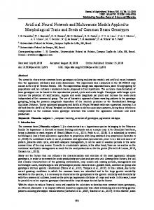
6.1 The Two-Spirals Problem (SPIR) Figure 4(a) illustrates the first problem tested, the so-called 2-spirals (SPIR) problem. This training set is composed of 190 samples in ℜ2 and aims at testing the capability of the networks to detect non-linearly separable clusters in low dimensional data. Figures 4(b) and (c) depict the MST and its corresponding histogram. From the MST histogram we can detect the existence of two different clusters in the network. In this case, the resultant memory matrix was composed of m = 121 antibodies, corresponding to a compression rate (reduction in the sample set size) CR = 36.32%. Note that the compression was superior in regions where the amount of redundancy is larger, i.e., the centers of the spirals (compare Figure 4(a) with 4(d)). SPIR

Minimal Spanning Tree (MST)

(a)

(b)

9

Final aiNet Structure

MST Histogram

1

2

(c)

(d)

Figure 4: aiNet applied to the 2-spirals problem. (a) 2-spirals problem (SPIR). (b) Minimal spanning tree, in which the dashed line represents the connection to be pruned. (c) MST histogram indicating two clusters. (d) Final network structure, determining the spatial distribution of the 2 clusters.

Figures 5(a) and (b) present the results for the SOFM with an initial number m = 121 output neurons, i.e., the same number of units as the aiNet. Sixteen output neurons not capable of classifying any input datum were pruned after learning (m = 105). The network final configuration and the resultant U-matrix (Ultsch, 1993) indicates the way the neurons were distributed. According to their neighborhood, the SOFM would not be able to appropriately solve this problem, since the final neighborhood configuration of the weight vectors leads to an incorrect clustering. SOFM Configuration

U-Matrix

(a)

(b)

Figure 5: Results obtained with the application of the SOFM to the SPIR problem. (a) Final network configuration and weight neighborhood, m = 49. (b) U-matrix.

6.2 The IRIS Data Set of Fischer The IRIS data set of Fischer is available for download in the Repository of Machine Learning Databases at the University of Irvine, California (URL 1). It is a real-world problem well-known and widely used to evaluate machine learning and classification capabilities of novel and stablished algorithms. The data set consists of M = 150 samples for three species (classes) of Iris: setosa, virginica and versicolor, with 50 samples in each class. All data have a dimension L = 4, i.e., there are four independent variables to be used in the learning process. These variables are measurements of the flowers, such as sepal and petal length. The data set is complete, in the sense that there is no missing attribute. 10

The aiNet has a plastic structure and a random learning procedure through clonal selection. Thus, each run of aiNet will present similar but slightly different results. Typical performances will be illustrated. The first aspect to be evaluated is the aiNet capability of learning and classifying the whole data set. Table 3 shows how the aiNet scales with relation to the suppression threshold (σs). It can be seen that for smaller values of σs, aiNet presents smaller compression rates but higher clustering capabilities. It is interesting to notice that class 1 (c1), that is linearly separable from the others, while classes 2 and 3 are not; suffers an improved compression, mc1 = 2 in all cases. This leads to the conclusion that the network is good at extracting information from this part of the data set. To quantify the aiNet percentage of correctly classified samples (PCC), the aiNet learning algorithm was applied, then the MST and hierarchical clustering techniques were used to determine which cells composed each of the three clusters. Figure 6 depicts the typical performance of aiNet for σs = 0.1. It can be seen from the MST histogram that nothing can be inferred concerning the number of classes in aiNet. In the previous example, SPIR, we concluded that the MST, and its corresponding histogram, is an interesting approach to detect clusters when there is a certain relative distance between the clusters, even if they are not linearly separable. This is also in accordance with the results presented in de Castro & Von Zuben (2000a). Nonetheless, this problem has also arisen when de Castro & Von Zuben (2001) applied aiNet to a benchmark task in which all classes constituted a single large class, i.e., there is no inherent separation between the many groups available in the data set. In that situation, the authors suggested the aiNet dendrogram as an alternative tool to detect and separate clusters. The only problem with this approach is the lack of an a priori knowledge of where to cut the dendrogram. If we cut the dendrogram of Figure 6(b) for the fusion value si,j ∈ [0.35,0.45] a correct cluster separation can be determined. After illustrating how to interpret the aiNet capability of detecting inherent cluster separation, it is important to test its generalization capability, i.e., its potential to respond to previously unseen data, or data not used during training. To do so, the IRIS data set was randomly split into two independent sets, each containing 50% of the whole data set, i.e., Mtr = 75 and Mte = 75. Table 3: aiNet performance for the IRIS data set. σs is the suppression threshold, Mm is the amount of misclassified samples, PCC is the percentage of correctly classified samples, mci , i = 1,2,3 is the number of memory antibodies for class i, m is the total number of memory antibodies (m = Σi mci), and CR is the aiNet compression rate.

σs

Mm

mc1

mc2

mc3

m

PCC (%)

CR (%)

0.05

7

2

19

21

42

95.33

72.00

0.10

10

2

14

18

34

93.33

77.33

0.15

16

2

6

10

18

89.33

88.00

0.20

29

2

4

6

12

80.67

92.00

11

aiNet Dendrogram 0.5

MST Histogram

0.45 0.4 0.35

si,j

0.3 0.25 0.2 0.15 0.1 0.05 0

(a)

(b)

Figure 6: aiNet typical performance for σs = 0.1. (a) MST histogram. (b) aiNet dendrogram.

Table 4 summarizes how the aiNet generalization capability scales with relation to σs for the test data set. From this table we can notice that the compression rate of aiNet is reduced for smaller values of the parameter σs. Figure 7 depicts the MST histogram and the aiNet dendrogram. It is interesting as, in this case, one can perceive the presence of three clusters in the MST histogram of Figure 7(a). There is a larger difference between one of the clusters and the other (II and III) and a smaller difference between the other two non-linearly separable clusters (I and II). Karayiannis and Mi (1997) reported that unsupervised clustering algorithms typically result in 1217 errors, what corresponds to a percentage of correctly classified samples on the order of 77.33%84%. These results are much inferior to those achieved by aiNet. The aiNet generalization capability is quite good even when compared with a supervised learning strategy. The best test performance reported by Karayiannis and Mi (1997) for a growing radial basis function (RBF) neural network was PCCte = 98.67%, a result comparable to the one presented by aiNet. The main difference was that his network reached a final architecture with m = 11 neurons (see Table V, in Karayiannis and Mi (1997)), while aiNet achieved a network with m = 60 cells for the same error rate. Although this difference in architecture complexity seems to be great, one must consider that the RBF network neurons are processing units, while the aiNet antibodies are information storage elements, as discussed in Section 5.

Table 4: aiNet generalization capability. σs is the suppression threshold, Mm is the amount of misclassified samples for the test set, PCCte is the percentage of correctly classified test samples, mci , i = 1,2,3 is the number of memory antibodies for class i, m is the total number of memory antibodies (m = Σi mci), and CRtr is the aiNet compression rate when compared to the size of the training set.

σs

Mm

mc1

mc2

mc3

m

PCCte (%)

CRtr (%)

0.05

1

16

19

26

60

98.67

20.00

0.10

2

7

13

15

35

97.33

53.33

0.15

2

5

7

8

20

97.33

73.33

0.20

4

4

5

7

16

94.67

78.63

12

aiNet Dendrogram 1 0.9

MST Histogram

0.8

I

II

III

0.7

si,j

0.6 0.5 0.4 0.3 0.2 0.1 0

(a)

(b)

Figure 7: aiNet performance for σs = 0.1. (a) MST histogram. (b) aiNet dendrogram.

7. Final Remarks and Future Trends In this paper, an artificial immune network model was discussed and mathematically detailed. The model is connectionist in nature but it follows an evolutionary-like learning algorithm, that is the immune clonal selection principle (Burnet, 1959). The motivation for the development of the immune network model, named aiNet, was stressed and it was theoretically and empirically compared with artificial neural networks. The theoretical comparisons allow us to conclude that there are many similarities between aiNet and ANNs and, certainly one area has much to gain from the other. Empirical results demonstrated the aiNet capability of solving non-linearly separable problems through the minimal spanning tree (MST) of a trained network, as far as there is a relative separation between the clusters. Otherwise, alternatives were given such that its performance could be evaluated and compared to other ANNs from the literature. It could be verified that, although it is a self-organizing strategy, its results were comparable to those obtained by one class of supervised learning algorithm for ANNs in classification problems. It is not difficult to speculate that powerful hybrid algorithms, combining immune network models and artificial neural networks, might soon arise. Additionally, we can propose as future extensions of this paper some enhancements and analysis of the aiNet model, like: 1) the development of a general framework to visualize a trained aiNet for network antibodies of length L ≥ 4; 2) a detailed convergence analysis of the algorithm; and 3) the inclusion of an affinity threshold ε, as suggested in Section 5.

Acknowledgments Leandro Nunes de Castro would like to thank FAPESP (Proc. n. 98/11333-9) for the financial support. Fernando Von Zuben would like to thank FAPESP (Proc. n. 98/09939-6) and CNPq (Proc. n. 300910/96-7) for their financial support.

13

References [1] Burnet, F. M. (1959), The Clonal Selection Theory of Acquired Immunity, Cambridge University Press. [2] Dasgupta, D. (Ed.) (1999), Artificial Immune Systems and Their Applications, Springer-Verlag. [3] De Castro, L. N., & Von Zuben, F. J. (2001), “aiNet: An Artificial Immune Network for Data Analysis”, submitted. [4] De Castro, L. N., & Von Zuben, F. J. (2000a), “An Evolutionary Immune Network for Data Clustering”, Proc. of the IEEE SBRN, pp. 84-89. [Online]

ftp://ftp.dca.fee.unicamp.br/pub/docs/vonzuben/lnunes/ainet.pdf [5] De Castro, L. N. & Von Zuben, F. J. (2000b), “The Clonal Selection Algorithm with Engineering Applications”, GECCO’00 – Workshop Proceedings, pp. 36-37. [Online]

ftp://ftp.dca.fee.unicamp.br/pub/docs/vonzuben/lnunes/gecco00.pdf [6] De Castro, L. N. & Von Zuben, F. J. (1999), “Artificial Immune Systems: Part I – Basic Theory and Applications”, Technical Report – RT DCA 01/99, p. 95. [Online]

ftp://ftp.dca.fee.unicamp.br/pub/docs/techrep/1999/DCA99-001.pdf [7] Fiesler, E. & Beale, R. (1996), Handbook of Neural Computation, Oxford University Press. [8] Haykin S. (1999), Neural Networks – A Comprehensive Foundation, Prentice Hall, 2nd Ed. [9] Holland, J. H. (1975), Adaptation in Natural and Artificial Systems, MIT Press. [10] Janeway, C. A., P. Travers, Walport, M. & Capra, J. D. (1999), “Immunobiology: The Immune System in Health and Disease”, 4th Ed, Garland Publishing. [11] Jerne, N. K. (1974), “Towards a Network Theory of the Immune System”, Ann. Immunol. (Inst. Pasteur) 125C, pp. 373-389. [12] Karayannis, N. B. & Mi, G. W. (1997), “Growing Radial Basis Neural Networks: Merging Supervised and Unsupervised Learning with network Growth Techniques”, IEEE Trans. on Neural Networks, 8(6), pp. 1492-1506. [13] Kohonen T. (1982), “Self-Organized Formation of Topologically Correct Feature Maps”, Biological Cybernetics, 43, pp. 59-69. [14] Kwok, T. Y. & Yeung, D. Y. (1997), “Constructive Algorithms for Structure Learning in Feedforward Neural Networks for Regression Problems”, IEEE Trans. on Neural Networks, vol. 8, n° 3, pp. 630-645. [15] Langman, R. E. & Cohn, M. (1986), “The ‘Complete’ Idiotype Network is an Absurd Immune System”, Imm. Today, 7(4), pp. 100-101. [16] McCulloch W. & Pitts W. (1943), “A Logical Calculus of the Ideas Immanent in Nervous Activity”, Bulletin of Mathematical Biophysics, 5, pp. 115-133. [17] Perelson, A. S. (1989), “Immune Network Theory”, Imm. Rev., 110, pp. 5-36. [18] Perelson, A. S. & Oster, G. F. (1979), “Theoretical Studies of Clonal Selection: Minimal Antibody Repertoire Size and Reliability of Self-Nonself Discrimination”, J. theor.Biol., 81, pp. 645-670. [19] Reed, R. (1993), “Pruning Algorithms – A Survey”, IEEE Trans. on Neural Networks, vol. 4, n° 5, pp. 740-747. [20] Ultsch, A. (1993), “Knowledge Extraction from Artificial Neural Networks and Applications”, Information and Classification, O. Optiz et al. (Eds.), Springer, Berlin, pp. 307-313. [21] _____ URL 1 Machine Learning Databases of the Institute of Computer Science of the University of Irvine, California [Online] ftp://ftp.ics.uci.edu/pub/machine-learning-databases. [22] Varela, F. J. & Coutinho, A. (1991), “Second Generation Immune Networks”, Imm. Today, 12(5), pp. 159-166.

14