TECHNICAL RESEARCH REPORT Implementation and Application of Principal Component Analysis on Functional Neuroimaging Data
by Fuad Gwadry, Carlos Berenstein, John Van Horn, Allen Braun
TR 2001-47
I R INSTITUTE FOR SYSTEMS RESEARCH
ISR develops, applies and teaches advanced methodologies of design and analysis to solve complex, hierarchical, heterogeneous and dynamic problems of engineering technology and systems for industry and government. ISR is a permanent institute of the University of Maryland, within the Glenn L. Martin Institute of Technology/A. James Clark School of Engineering. It is a National Science Foundation Engineering Research Center. Web site http://www.isr.umd.edu
IMPLEMENTATION AND APPLICATION OF PRINCIPAL COMPONENT ANALYSIS ON FUNCTIONAL NEUROIMAGING DATA Fuad G. Gwadry*, Carlos A. Berenstein, John D. Van Horn and Allen R. Braun
The work of F. G. Gwadry and C. A. Berenstein was partially supported by grants from The National Science Foundation (DMS-9622249; DMS-0070044). Asterisk indicates corresponding author. Email:
[email protected] *F. G. Gwadry is with the Laboratory of Molecular Pharmacology, Division of Basic Sciences, National Cancer Institute, National Institutes of Health, Building 37, Room 5D02, 37 Convert Dr., Bethesda, MD 20892 and with the Department of Mathematics and Institute for Systems Research, University of Maryland, College Park, MD 20742. J. D. Van Horn is with the Laboratory of Brain and Cognition, NIMH, National Institutes of Health, Building 10, Room 4C-104, 9000 Rockville Pike, Bethesda, MD 20892. C. A. Berenstein is with the Department of Mathematics and Institute for Systems Research, University of Maryland, College Park, MD 20742. A.R. Braun is with the Language Section, VSLB/NIDCD, National Institutes of Health, Building 10, Room 5N18, 9000 Rockville Pike, Bethesda, MD 20892.
Abstract --Recent interest has arisen regarding the application of principal component analysis (PCA) -style methods for the analysis of large neuroimaging data sets. However, variation between different implementation of these techniques has resulted in some confusion regarding the uniqueness of these approaches. In the present article, we attempt to provide a more unified insight into the use of PCA as a useful method of analyzing brain image data contrasted between experimental conditions. We expand on the general approach by evaluating the use of permutation tests as a means of assessing whether a given solution, as a whole, exposes significant effects of the task difference. This approach may have advantages over more simplistic methods for evaluating PCA results and does not require extensive or unrealistic statistical assumptions made by conventional procedures. Furthermore, we also evaluate the use of axes rotation on the interpretability of patterns of PCA results. Finally, we comment on the variety of PCA-style techniques in the neuroimaging literature that are motivated largely by the kind of research question being asked and note how these seemingly disparate approaches differ in how the data is preprocessed not in the fundamentals of the underlying mathematical model. Index terms -- Principle component analysis; neuroimaging; mathematical model; statistics; permutation tests; brain activation
I. INTRODUCTION Current methods for the analysis of functional neuroimaging data rely principally upon performing voxel-wise univariate test statistics across the brain [1]. Using this approach, researchers can identify regionally specific areas of significant change in the pattern of brain blood flow response between behavioral or cognitive task conditions. However, under this univariate framework little consideration is given to the functional inter-relations amongst voxels located in distributed brain areas. With this in mind, multivariate approaches for analyzing functional neuroimaging data have been recommended by several research groups [2],[3],[4],[5],[6],[7],[8]. These authors have utilized several variations of principal component analysis (PCA) in order to extract different features from the covariance or correlation matrix. For instance, Clark et al. [2] applied PCA to the intersubject correlation matrix, a method known as Qcomponent analysis in the statistical literature, in order to identify subtypes of individuals. Moeller and colleagues have advocated the use of the scaled subprofile model (SSM) [3],[4],[6],[7],[8] which, following a logarithmic transformation of the image data, involves applying PCA to the subject-region interaction term in order for the components to represent systematic differences in brain function among subjects and/or groups. Friston et al.’s [5] eigenimage analysis performs singular value decomposition (SVD) of the overall data matrix, while more recently, McIntosh et al. [9] have applied the partial least-squares (PLS) method involving the cross-correlation of the image data with the experimental design matrix. All in all, the general theory underlying PCA decomposition of large datasets has not been satisfactorily presented and, moreover, the variations on this general approach that exist in the literature may have lead some to believe that these methods are not related. Therefore, we believe that the general method for PCA requires a more complete mathematical description in addition to it being shown how the solutions derived from PCA may be improved upon using methods of axis rotation and may be assessed for statistical relevance using permutation testing. This is the aim of the present article in which we detail and apply these concepts to a large postitron emission tomographic (PET) data set acquired under two cognitive stimulation conditions. II. THEORY AND ASSUMPTIONS A. Principal Component Analysis (PCA) The Pre-PCA data processing steps are outlined below in the Methods. The processing included the derivation of the difference image matrix. PCA or equivalently, in this case, singular value decomposition (SVD), was applied to the M × N difference matrix X with elements xij
(i = 1,2,.., M ; j = 1,2.., N ) , where M
is the number of subjects and N is the number of voxels.
xi• . Because the number of rows M is less than the number of columns N , the rank of X is equal to M . The SVD of X is given by:
Therefore, each subject’s difference scan is represented by
X = USV T
(1)
where: (i)
U and V are (M × M ) and ( N × M ) , respectively, each of which have orthonormal columns
(ii)
U T U = I , and V T V = I ; S is an (M × M ) diagonal matrix with its diagonal elements in descending order of magnitude;
(iii)
and superscripted “T” denotes transposition.
so that
The columns of V are termed the right singular vectors or principal components (PCs) consisting of the voxel loadings. The columns of U are the left singular vectors consisting of the subject loadings for
3
each of the PCs. The diagonal elements of S are the singular values or variances1 for each of the PCs. For a more thorough description of SVD for functional neuroimaging data see Friston et al. [5]. It should be emphasized that voxels across subjects were not standardized to have means of zero and standard deviations of one as has been required elsewhere (e.g., [10]). Variances were not unitized since one can assume that all the data elements are measured in the same metric. Also, we were interested in the differences between voxel variances. In the case of an image difference matrix, subtracting voxel means across subjects (i.e., centering) would remove the general (consistent) characteristics or effects of the state or task transition, and would limit one to seeing patterns of individual differences in these effects. By analyzing non-centered differences, it is possible to see and extract each pattern relative to its true baseline rather than relative to the mean across differences. The components then represent patterns of activation shifts that do not have the same relative size from one subject to another. Centering has the effect of removing the overall mean contrast effect(s) and probably changing the relative variance attributed to different components underlying the differences. In the next section we describe a cutoff criterion for the number of significant components by identifying the pattern of data variation that is significant from noise. By using permutation tests we were able to assess the significance of PCs without relying on the distribution assumptions underlying most conventional parametric statistical methods. B. Singular Value Significance Determined Using Permutation Tests Use of standard significant tests for determining the number of PCs to retain introduces assumptions that the principal component model itself does not require. For example, multivariate normality as well as independence of errors are assumptions of multivariate tests of significance (e.g., [11]). These methods rely on parametric assumptions that may be possibly false, and on various approximations, which may not be appropriate for the data at hand. Moreover, PET studies generally consist of small number of data sets that may result in departures from the assumptions [12]. Randomization and permutation methods do not require elaborate statistical assumptions made by conventional approaches; that is, no expectations about the distributional nature of the data is required since no reference is made to a theoretical model. Moreover, these tests have the important statistical advantage of consistently protecting against Type 1 error rates (i.e., the probability of rejecting the null hypothesis when, in fact, the null hypothesis is true). They are also valid without a random sample, although generalizations from these tests on a particular sample may be constrained by the sampling procedure [13],[14]. Since PCA treats the data as consisting of a single sample, randomizing the order of subjects would not change the calculations in any way. Also, randomly permuting the assignments of conditions for the two scans involved in a given subject contrast will not change the singular values or other measures of fit. This makes sense when one considers the fact that exchanging assignments of scans to the two experimental conditions in a given contrast does not change the interrelationships among variations across the voxels; it merely reverses the signs of the subject loadings on a given component. On the other hand, randomly permuting the signs of the voxels of a contrast image may yield the strongest inferences that a “real” component or factor is in fact a consequence of the task or activation state change. To test for the number of components to retain, one would sequentially compare the residual variance after each component extraction of the unpermuted (original data) with the randomly permuted versions of the data. Significance level or probability value would be computed as the proportion of data permutations, including the one representing the unpermuted results that have test values greater than or equal to the value of the unpermuted results. For example, in order to test at a significance level of 0.001, one would have to permute the data 999 times (i.e., 1/1000). One would sequentially test in this fashion until the residual matrix is found to contain no significant variance. At this point the correct number of components have been extracted. Note that only signs of the voxels from the difference images would be
1
The variances are computed as the squared singular values over the sum of the squared singular values in
S ; that is, σ • j = diag ( s 2j ) / trace( s 2j ) . 4
randomly permuted. The position of the voxels would not be permuted in any way. Permuting the position of voxels in an image would violate any expected spatial relationships among the voxels. The random permutation of the signs of the voxels must be performed on the unthresholded difference images prior to any smoothing in order that the residual variance after each successive extraction can be accurately tested. Permuting the signs of voxels from the smoothed difference images would remove the expected spatial correlations among voxels, due to the smoothing procedure, that would exist even independently of task or state changes in the subjects. As a result, permuting voxels in the smoothed images would be unrealistic because the “null image” would be too uncorrelated. After the random permutations, the differences can be smoothed before any principal component decomposition2. C. Analytic Rotation of PCs In standard principal component analysis (PCA) and factor analysis (FA), it is customary to rotate the reduced set of components or factors to some kind of “simple structure”. This is generally done using Kaiser’s [15] varimax procedure. The simple structure criteria is used to overcome rotational indeterminacy of the components or factors. This is achieved by rotating the components or factors so that each variable loads on as few components or factors as possible (cf. [16]; pp. 177-212). The orthogonal rotation for simple structure applies these restrictions while simultaneously restricting the transformation matrix so that the components or factors remain uncorrelated. Oblique simple structure relaxes the requirements of orthogonality of axes. Kaiser’s [15] varimax procedure finds an orthogonal transformation or rotation matrix Trr such that the variance (i.e., sum of squares of variable loadings) is maximized across all components or factors in the matrix. In order that variables with higher average loadings than others do not overly influence the final rotated solution, Kaiser reformulated his criterion so that each row of the component or factor matrix is rescaled to have unit sum of squares; thus giving equal emphasis to all rows (i.e., variables). After the rescaled matrix is varimax rotated, the original row scales are then restored. This procedure is routinely implemented with varimax rotation and is referred to as Kaiser-normalization. Harris and Kaiser [17] further developed a two-stage procedure that starts with an orthogonal rotation, such as varimax, and extends it to an oblique solution. Since the rotation involves a combination of orthogonal and oblique solutions, it is referred to as orthoblique. This is the approach used here and is accomplished as follows: In accordance with the definition of orthogonality, all orthogonal transformation matrices have the following characteristics:
Trr T T rr = I rr = T T rr Trr
(2)
where r is the number of PCs retained after, in this case, permutation testing. Because equation (2) equals the identity matrix, it can be substituted in equation (1) without influencing the ability of the derived singular values (variances) and vectors (subject and vowel loadings) to reproduce the original data matrix. That is, applying a rotation or transformation matrix may shift the size (variances) of the components or factors, but the set of new (rotated) components or factors will retain the same ability to reproduce the original data matrix. The reproduced data matrix as a function of the singular values and vectors from equation (1) is:
Xˆ mn = U mr S rrV T rn where
(3)
U mr and Vnr are the truncated left and right singular vectors, respectively, and S rr contains their
singular values. Then substituting equation (2) into the middle of equation (3) and adding parentheses gives:
2
Theoretically one should also take into account the spatial correlations as a result of the registration and stereotaxic normalization of the scans. However, this issue could not be addressed in the same manner.
5
(
)(
p 1− p Xˆ = U mr S rr Trr T T rr S rr V T rn
)
(4)
where: (i) the power of p is the user defined parameter (ranging from 0 to 1.0) that influences the degree of correlation allowed among the components or factors; and (ii)
p
S rr and S rr
1− p
replaces
S rr .
We can then define the rotated versions of
U mr and Vnr as:
~ p U mr = U mr S rr Trr
(5)
~ 1− p Vnr = Vnr S rr Trr
(6)
Trr is the orthogonal varimax transformation matrix defined in equation (2). ~ When p is set to 0 the components are restricted to be uncorrelated; that is, the columns of U are orthogonal. Values of p between 0 and 1 produce more highly correlated solutions. When p is set to 1, all ~ orthogonality restrictions are omitted (i.e., the vectors in U are correlated). ˜ and is absorbed into V˜ . A After the components are rotated, the scale is removed from U ˜ is created, i.e., diagonal matrix of the square root sum of squares of the columns of U 1/ 2 M ~ 2 D = diag ∑U ij . The scale in U˜ is removed by post-multiplying U˜ by the inverse of D ; that is, i =1 ˜˜ ˜ −1 U = U˜ D , such that the columns of U˜ are unitized. The scale is absorbed into V˜ by post-multiplying V˜ ˜ ˜ by D ; that is, V˜ = V˜D , where the column sum of squares of V˜ over the trace of the squared singular values in S are equal to the proportion of variance accounted for by each rotated component. where
III. MATERIALS AND METHODS A computational flowchart of the steps involved is illustrated in Figure 1. A. Data Acquisition 1) Subjects Informed consent was obtained from all 19 subjects after the risks, hazards and discomfort associated with these studies were explained. The 19 subjects included 8 females [age: 36 ± 10 years (Mean ± SD), range 24 -50] and 11 males [34 ± 8, range 23-47]. Each subject performed all skilled manual functions (writing, throwing a ball, combing, using scissors or other tools, etc.) with the right hand. All subjects were free of medications at the time of the scan. 2) Scanning Methods PET scans were performed on a Scanditronix PC2048-15B tomograph (Uppsala, Sweden) which has an axial and in-plane resolution of 6.5 mm. Fifteen slices, offset by 6.5 mm (center to center), were acquired simultaneously. Subjects eyes were patched, and head motion was restricted during scans with a thermoplastic mask. For each scan, 30 mCi of H215O were injected intravenously. Tasks were initiated 30 seconds prior to injection of the radiotracer and were continued throughout the scanning period. Scans commenced automatically when the count rate in the brain reached a threshold value (approximately 20
6
seconds after injection) and continued for 4 minutes. Emission data were corrected for attenuation by means of a transmission scan. Arterial blood was sampled automatically during this period, and PET scans and arterial time activity data were used to calculate cerebral blood flow images with a rapid least squares method [18]. 3) Experimental Task Paradigm The experimental paradigm consisted of (1) a narrative speech condition in which subjects were instructed to spontaneously recount an event or series of events from personal (episodic) memory, using a normal speech rate, rhythm and intonation where semantic content was typically rich in visual detail; and, (2) a resting task condition, in which subjects were given no explicit instructions and were to lie still without speaking or moving for the duration of the scan period. These task conditions were presented in a counterbalanced order across the 19 subjects. For a more detailed description of the overall experimental design see [19]. B. Image Processing 1) Registration and Preprocessing Following data collection, the PET scans were registered using Statistical Parametric Mapping (SPM) software [20]. The 15 original PET slices were interpolated and spatially registered in order to minimize the effects of head movement, and stereotaxically normalized to produce images of 26 planes parallel to the anterior-posterior commissural line in a common stereotaxic space [21] cross-referenced with a standard anatomical atlas [22]. 2) Thresholding and Proportional Scaling The 65 × 87 × 26 images from each the experimental conditions (i.e., narrative speech and rest) were vectorized in order to create a voxel-by-subject image matrix for each condition. The dimensions of each of these matrices were then 147030 × 19 . Images were thresholded (i.e., voxels with numerical values falling within a predetermined range were selected) and then proportionally scaled. Two thresholds were applied in order to select voxels that only represented gray matter. Thresholding and proportional scaling procedures were performed as follows: (1) Images were smoothed using a 3D Guassian filter with full width at half maximum (FWHM) values of 20 × 20 × 12 mm for x , y and z axes, respectively; (2) A mean over all voxels greater than one-eighth of the mean computed over the entire image was derived for each image; (3) In order to be selected, a given voxel had to be greater than 80% of the mean computed in the proceeding step and had to meet this criteria for all images. These voxels were considered to most reliably represent gray matter; (4) An index of the location of the voxels selected was then saved for subsequent steps in the analysis; (5) The global CBF value for each of the unsmoothed images was then estimated as the mean of the gray matter voxels indexed in the preceding step; (6) Each of the unsmoothed images were proportionally scaled by dividing each voxel value by it’s estimated global CBF. It is worth noting that the method in which the images were thresholded and proportionally scaled was similar to what is done in SPM [20]. The differences between the two approaches is the derivation of the global CBF and the position of the proportional scaling step. In SPM the global CBF used to proportionally scale each image is the mean computed in Step 2 above. After the images are proportionally scaled, voxels that do not exceed 0.80 (or some user defined threshold) for all images are thresholded out. In the current analysis, voxels had to meet both threshold criterion across all images in order to be included in the derivation of the global CBF. As a result, the global CBF was based on the same voxels across all images. This was considered a more precise method of estimating gray matter CBF. The proportionally scaled unsmoothed images were then subtracted from one another, i.e., a narrative minus rest difference images were derived. We derived the difference images before smoothing because permutation of the signs of the voxels had to be done on the unsmoothed images for reasons outlined in the Theory.
7
C. Statistical Analysis 1) Singular Value Significance Determined Using Permutation Tests The random permutation test to determine the number of components to retain was performed on the image difference matrix. The random permutation test procedure is described by the following steps: (1) 999 versions of the unthresholded unsmoothed image difference matrix were generated by randomly permuting the signs of the voxels 999 times using the uniform random number generator in MATLAB (Version 4.2, Mathworks, Natick, MA); (2) In order to investigate the influence of image smoothing, the data were then smoothed with one of two 3D Gaussian filters ( 20 × 20 × 12 or 10 × 10 × 6 mm for x , y and z axes); (3) Gray matter voxels were then selected; (4) The singular values of all 1000 data sets were extracted; (4) For each data set the proportion of total variance was computed by dividing the squares of the singular values for the components extracted by the total sum of the variances (i.e., the sum of the squared singular values); (5) The variances for the first components extracted from the 999 permuted data sets were compared to the variance for the first component extracted from the unpermuted data set in order to determine significance. The value was computed as the proportion of all 1000 data sets that had variance values greater than or equal too the value extracted from the unpermuted data set. The minimum probability value that could occur was 0.001; (6) After the variance of the first component extracted was tested, significant tests of the residual variances after each additional component extraction were performed. The maximum number of components were extracted from the data in each case in order to study the curve of the residual variances across successive component extractions. In practical applications, one would only sequentially test the residuals until one is found to be nonsignificant. The number of components already extracted would then be designated as the number to retain. The steps outlined above were also carried out on synthetic data derived as follows: Two 147,030 by 19 random data matrices were derived using the uniform random number generator in MATLAB; (2.) The index derived from the narrative minus rest data set was used to proportionally scale the randomly generated data; (3) The proportionally scaled matrices were then subtracted from one another. As with the case of the narrative minus rest data set, two different levels of smoothing were used. Since a series of significant tests are computed, the overall significance level of the sequence of tests is not the same as the individual significance levels of each test. Furthermore, the number of tests done is random and not fixed, and the tests are not independent of each other. To address this, the final significance levels incorporated the Bonferroni correction for multiple comparison by simply multiplying each observed probability value by the number of tests performed. D. PCA Output 1) Analytic Rotation of PCs After the number of components to retain was determined, the selected components were rotated using Harris and Kaiser’s [17] generalization of varimax with Kaiser normalization [15]. The components were allowed to be fully oblique; that is, the parameter p was set to 1 (see Theory). The rotated versions of the subject and voxel loading matrices were further transformed. The scale in the subject loading matrix was absorbed into the voxel loading matrix. Then the scale of the subject loading matrix was removed by rescaling the columns to have unit sum of squares. Also, if the sum of cubes of the subject loadings were negative for a given component, the signs of the subject loadings and corresponding voxel loadings for that component would be reflected. 2) Component Images In order to display the components as images, it was necessary to move the voxel loadings back to their original spatial coordinates. This was done by using the index of locations for the voxels retained for analysis. Interpretation of component images was facilitated by separating negative and positive voxel loadings and then displaying them on a standardized MRI scan. The MR image were transformed linearly into the same stereotaxic (Talairach) space as the PET. Using Voxel View Ultra (Vital Images, Fairfield, Iowa), component and MR data were volume-rendered into a single three-dimensional image for each group. The volume sets were resliced and displayed at selected planes.
8
IV. RESULTS The findings will be presented in detail in order to illustrate each of the computational steps shown in Figure 1. The total number of voxels retained after thresholding was 54, 358 of 143,030 voxels. The threshold criterion were applied to the 20 × 20 × 12 mm smoothed images in order to increase the relative signal to noise in the unsmoothed data. So that the number and location of voxels would not be a confound in the analysis the same voxels identified as gray matter voxels from the 20 × 20 × 12 mm smoothed data were also used for the analysis of 10 × 10 × 6 mm smoothed data. A. Permutation Test Figure 2 is a plot of the percent of variance for the first components extracted and the percent of residual variances for each subsequent component extracted from the 999 permuted data sets and the unpermuted data set for each of the two levels of smoothing (FWHM values of 20 × 20 × 12 mm and 10 × 10 × 6 mm). Filter size had an influence on the number of components found to be significant by the random permutation test. When this test was applied to the data having FWHM values of 20 × 20 × 12 mm (Figure 2a) it showed that five components could be extracted from significant variance (corrected P ≤ 0.05 ). However, when FWHM values of 10 × 10 × 6 mm were applied to the data (Figure 2b), it showed that only two components could be extracted from significant variance (corrected P ≤ 0.05 ). The correlations between the first five unrotated components extracted from the 10 × 10 × 6 and 20 × 20 × 12 mm smoothed data were assessed and are summarized in Table 1. The correlation table shows that the first extracted components were congruent with one another with a correlation of 0.898. In addition, PCs 2, 3 and 5 from the 10 × 10 × 6 mm smoothed data set corresponded with PCs 2, 3 and 4 from the 20 × 20 × 12 mm smoothed data set, respectively, with absolute correlations in the range of 0.721 to 0.763. Although the correlation between PC4 from the 10 × 10 × 6 mm smoothed data with PC5 from the 20 × 20 × 12 mm smoothed data was only 0.478, there were no competing correlations indicating that the two components do indeed correspond to one another. As illustrated in Figure 2, filter size also effected the variability of the variance values of the permuted data sets at each component level. As filter size increased, fluctuations in the variance values of the 999 permuted data sets increased as well. Moreover, the magnitude of the percent of variances for the first several components extracted from the permuted and unpermuted data sets increased as a function of filter size. This is more apparent for the component variances extracted from the unpermuted data set. For example, the first five component variance values extracted from the 10 × 10 × 6 mm smoothed data were 23.97, 9.54, 9.26, 9.13 and 9.73, respectively (Figure 2b). On the other hand, the component variance values extracted from the 20 × 20 × 12 mm smoothed data were 37.73, 16.13, 14.57, 14.44 and 12.32, respectively (Figure 2a). In order to evaluate the findings above, the random permutation test was applied to a synthetic data set. Figure 3 illustrates the variance curves extracted from the synthetic random set. The variances extracted from the 999 permuted data sets and the unpermuted data sets for each level of smoothing are plotted. The shape of the curves extracted from the permuted real data sets in Figure 2 are not evidently different from the curves extracted from the permuted and unpermuted synthetic data sets. Consistent with what was observed in the analysis, fluctuations in the variance values of the 999 permuted data sets increased as a function of filter size. Moreover, the magnitude of the percent of variances extracted from both of the data sets increased as a function of filter size. Large changes in percent of variances extracted from the unpermuted synthetic data set was not observed since by virtue of the data no structure exists. In both the real and synthetic case the means, standard deviations of and the minimum percent of variance values extracted from the 20 × 20 × 12 mm smoothed data set were always greater than or equal to the percent of variance values extracted from the 10 × 10 × 6 mm smoothed data set. This was also the case for the percent variance values extracted from the unpermuted data sets. B. Analytic Rotation of PCs After determining the number of components that contain significant variance, the reduced set of components extracted from the unpermuted 20 × 20 × 12 mm smoothed thresholded image difference
9
matrix were obliquely rotated. The five obliquely rotated components extracted from the 20 × 20 × 12 mm smoothed data set are displayed on a standardized MRI scan in Figure 4. The total solution accounted for 66.53 % of the total variance. Each of the five rotated components accounted for 21.45, 10.66, 8.77, 8.32 and 17.33 percent of the total variance, respectively. Moreover, each of the five components before rotation accounted for 37.73, 10.05, 7.61, 6.44 and 4.70 percent of the total variance, respectively. The rotational procedure spread out rather large proportions of the variance from the first component to the fifth component. This is illustrated by the proportional changes in variances accounted for by each component after rotation: 0.57, 1.06, 1.15, 1.29 and 3.69. As outlined in the theory, the rotational procedure does not effect the total amount of variance of a particular solution, but rather redistributes the variances across the set of components. The effects of rotation on the distribution of the components is also illustrated by the correlations between the unrotated and obliquely rotated components summarized in Table 2. The correlation table shows that only two of the five components are congruent with one another. Unrotated PCs 2 and 4 match with obliquely rotated PCs 2 and 4 with absolute correlations of 0.880 and 0.810, respectively. Also, despite the correlation between unrotated and rotated PC1 of 0.705, there were appreciable competing correlations between unrotated PCs 1 and 5 with rotated PCs 5 and 1 with correlations of 0.591 and 0.567, respectively. The correlations between unrotated PC1 and rotated PC5 again suggest that the rotational procedure distributed the variance from the first component to the fifth component. Table 3 summarizes the interrelationships between the five obliquely rotated components - which is reflected in terms of the correlation between the subject loadings for each of the PCs. The correlation table shows that the most appreciable correlations from highest to lowest were between PC2 and PC5 with a correlation of -0.367; PC1 and PC4 with a correlation of -0.321; between PC1 and PC5 with a correlation of -0.291; and finally between PC1 and PC2 with a correlation of -0.224. The correlations among the other components were in the absolute range of 0.006 to 0.117. C. Subject Loadings A plot of the subject loadings with respect to a pair of PCs can be used to detect outliers in the data set; that is, observations that are inconsistent with the remainder of the data. Figure 5a shows a plot of the subject loadings for the first and second unrotated components extracted from the 20 × 20 × 12 mm smoothed data set. The plot indicated no outliers were present in the data. In addition, a two-dimensional plot of the subject loadings can also be useful in identifying clusters or "types" of individuals. The PCs may provide a basis in which the subjects are clustered. For example, the two-dimensional plot of the subject loadings for the first and fifth obliquely rotated components illustrated in Figure 5b show two clusters of subjects. The plot shows that there are at least two clusters of individuals, one consisting of seven of the eight females and three of the eleven males in the sample. The other cluster consists of one of the eight females and eight of the eleven males in the sample. D. Effects of Mean Centering In order to examine the effects of centering on the components, the correlations between the first five unrotated components extracted before centering and after centering were assessed and are summarized Table 4. The correlation table shows that only three of the five components extracted are congruent with one another. PCs 2, 3 and 4 from the uncentered data matched PCs 1, 2 and 3 from the centered data, respectively, with absolute correlations ranging from 0.813 to 0.867. The first five components extracted from the centered data accounted for a total of 53.00 % of the total variance, as compared to 66.53 % from the uncentered data. Each of the five components accounted for 16.04, 11.93, 10.07, 7.66 and 7.30 percent of the total variance, respectively. Centering changed the relative variance attributed to the different components underlying the contrast. This is illustrated when one considers the proportional changes in variance accounted for by each component after centering: 0.425, 1.187, 1.323, 1.190 and 1.553. Centering placed less emphasis on PC1 in terms of variance accounted for. Also, there were no apparent matches between PCs 1 and 5 from the uncentered data with PCs 4 and 5 from the centered data. It is interesting to note that when the random permutation test was applied to the 20 × 20 × 12 mm smoothed centered data, the random permutation test ( N = 999 ) clearly showed that only three components could be extracted from significant variance (corrected P ≤ 0.05 ; not shown here).
10
V. DISCUSSION There are several distinctions in the present application that differ from previously reported approaches. First of all, PCA is applied directly to a difference matrix. This was also the case in more recent applications of SSM in which PCs were computed from a subject-region interaction term of a difference matrix [10],[23]. As described above (see Theory) we wanted to maintain subject-region main effect(s) and therefore did not center the data in any way. McIntosh et al.’s [9] application of PLS is similar to this since the design matrix represented contrasts between experimental conditions. Because the PCs were computed from cross-products rather than covariances the data were also not centered in any way. Secondly, we describe a statistical method of determining the number of significant PCs without relying on distributional assumptions underlying many conventional parametric statistical tests. For instance, the permutation test employed by McIntosh et al. involves reordering the rows of the design matrix so that associations of experimental conditions with images are destroyed and after each ordering, computing a new SVD and a new ANOVA on the analogous scores. In the single contrast case, this would be equivalent to permuting the assignments of conditions for the two scans involved in a given subject contrast. In our analysis this would not change the singular values or other measures of fit (see Theory). Under the SSM approach a statistical method (based upon Mauchley's sphericity test) for determining the number of PCs to retain has been suggested [3],[4],[6] that assumes multivariate normality, as well as independence of errors, but has not been consistently employed in recent applications of SSM. For example, some studies have applied Cattel’s scree test [24] to determine the number of PCs [25],[26] or have arbitrarily chosen the cutoff for the number of PCs [27],[10],[28] that require a degree of subjectivity. However, selection of SSM PCs based on the strength of their relation to behavioral measures of task performance has been recently applied [23]. Thirdly, other approaches discussed above have relied upon interpretation of the unrotated PC solution whereas we apply an analytic rotation to simple structure. Further, since the components may represent brain structures that are probably functionally related in varying degrees, we relaxed all orthogonality restrictions. This may be a better estimate of the component structure minimizing distortions that might occur in a more restrictive orthogonal rotation. We are then able to look at interrelationships between the brain structures or components that would not have been evident with the original, unrotated solution. To our knowledge, this is the first application of analytic rotation to the reduced set of PCs computed from voxel-wise functional neuroimaging data. A. Singular Value Significance Determined Using Permutation Tests Randomization or permutation methods have been used by several research groups for testing the mean differences between neural images, including PET, MRI and EEG maps [29],[12],[30]. In the current case, permutation methodology was used to determine the number of significant PCs. As shown in Figure 2 filter size had an influence on the number of components found to be significant by the permutation test. When the data were smoothed with the larger filter the permutation test showed that five components could be extracted from significant variance; however, when the data were smoothed with the smaller filter it showed that two components could be extracted from significant variance. The congruence between most of the components from the two solutions suggest that increasing the filter size did not dramatically alter the pattern of the components themselves (Table 1). Figure 2 also shows that as filter size increased fluctuations in the variance values of the permuted data sets increased as well. This was reflected by the fact that the variance values extracted from the data smoothed with the larger filter had means, standard deviations and minimums greater than or equal to the variance values extracted from the data smoothed with the smaller filter size. This relationship was also observed from the variance curves extracted from the synthetic data set shown in Figure 3. This supports the contention that the relationship is indeed real and is not an artifact inherent in the real data set. As indicated in the literature, an “optimal” level of image smoothing is difficult to determine and, moreover, a constant level of smoothing may not be suitable for measuring maximal signal in all brain areas simultaneously [31]. These observations imply that the differences in pattern obtained between the two smoothing levels presented here may not persist as smoothing filter is varied further. One way to investigate this would be to smooth across different levels that may give an indication of the optimal level of smoothing needed to maximize loadings in certain brain regions. However, the two smoothing kernel sizes chosen here are the two most commonly used for PET imaging data and further examination of issues related to image smoothness, though of fundamental importance, are beyond the scope of this article.
11
B. Analytic Rotation of PCs The previous PCA studies cited above have relied on the unrotated components for interpretation. The unrotated PCs are orthogonal and ordered in decreasing magnitude of variance accounted for. In the current case, the reduced set of components were rotated using Harris and Kaiser’s generalization of varimax [17] with Kaiser normalization [15]. A rotation position is sought where the variance is maximized across all components in the matrix. The rotational procedure does not effect the total amount of variance accounted for by a particular solution, but rather redistributes the variances across the set of components. Our findings showed that the rotational procedure spread out rather large proportions of the variance from the first component to the fifth component (Table 3). This was also illustrated by the proportional changes in the variances accounted for by each component after rotation. The correlations between the unrotated and rotated solutions also show that only two of the five components had appreciable correlations between one another; thus, suggesting that rotation did make considerable changes to the distribution of the variance. An advantage of Harris and Kaiser’s generalization of varimax [17] is that it provides a means for determining whether the components are indeed orthogonal or oblique. One could vary the parameter p systematically from 0 to 1 and select the solution that has the simplest and most theoretically meaningful pattern. If the correlations among the oblique components are negligible, then the orthogonal solution would be more reasonable. Since in this case the components may represent brain structures which are probably all functionally related to varying degrees, it is likely that the components will not be statistically independent. Therefore, oblique rotations may be better estimates of the component structure, minimizing distortions which might occur in a more restrictive orthogonal rotation. We are then able to look at interrelationships between the rotated components. Our findings show some interrelationships between the components extracted, namely, PC2 and PC5, PC1 and PC4, PC1 and PC5, and PC1 and PC2 (Table 4). These patterns may be taken as illustrating how the sensory motor and language like components interact with one another. C. Mean Centering As noted earlier, the data were not centered in any way in order to maintain the overall mean contrast effect(s). Centering across subjects, as would be the case if the PCs were computed from the correlation or covariance matrix, would remove the general (consistent) effects of the task transition and would limit us to seeing patterns of individual differences in these effects. Also, different components can be uncovered by different centerings. The relative emphasis of the components before and after centering was assessed by comparing the relative variance attributed to the uncentered components to their centered components. It was found that centering placed less emphasis on PC1. Moreover, when the correlations between the first five unrotated components before and after centering were assessed (Table 5) there were no apparent matches between PCs 1 and 5 from the uncentered data with any of the PCs from the centered data. It is interesting to note that when the random permutation test was applied to the centered data, three components were found to be significant. The first three unrotated PCs extracted from the centered data corresponded with PCs 2, 3 and 4 from the uncentered data. The lack of correspondence between PCs 1 and 5 from the uncentered data with any of the PCs extracted from the centered data, and the proportional changes in variance of PC1 after centering shows how some components can be discarded in the centered versus uncentered solutions. Tucker [32] points out that centering of the data before PC decomposition is analogous to rotation of axes in component and factor analysis. Geometrically, after centering, the axes are parallel to the corresponding axes before centering; they have simply been translated as a unit from the original origin to a new origin at the centroid of the configuration. One can then easily derive the centered solution from the uncentered, and visa versa, with a suitable rotation to restore the equivalence of axis orientation in factor space. The above discussion shows that the effects of different centering schemes are quite straightforward. Nonetheless there has been considerable controversy on this point, with some authors claiming that different (or novel) components can be uncovered (or revealed) by different centering approaches (e.g., [2],[3]). One reason that some investigators have gotten this impression is that different centering schemes can give different relative emphasis to the dimensions underlying the data set; the relative emphasis before and after centering is determined by the relative sizes of the sum of squares of their original loadings compared to their centered loadings (i.e., variances). This change in sum of squares will change the relative contributions of the dimensions to each unrotated component. If some components are
12
discarded to obtain a lower dimensional solution, then different parts of the factor space may be discarded in the centered versus the uncentered solutions. PCA of uncentered data will have large first components due to the presence of means. The consequence of removing any mean is that the amount of total variation explained by a particular analysis will be smaller and sometimes dramatically smaller. Therefore, different centering can give different relative emphasis to the components underlying the data set. The situation with variances is similar. One could consider standardizing the overall variance to unity over the entire data set, but this has no influence on the outcome of the analysis because all the data values are divided by the same constant. The fundamental difference between centering and standardization is that combinations of different centering methods do not influence each other, while standardizations do. For instance, double-centering can be done separately and in any order. For standardization, the situation is however far more complex: standardization of one mode will generally destroy that of another. For the cases cited above, the kind of research question being asked determined what was done with the row or column means, or main effects to retain for analysis. In certain cases with homogeneous variables the differences in the means are of interest, and should be retained for analysis. The situation with variances is similar. D. Subject Loadings A plot of subject loadings with respect to a pair of PCs, when derived from an uncentered matrix, can be used to detect outliers in the data set; that is, observations which are inconsistent with the remainder of the data. The plot of the subject loadings for the first and second unrotated components extracted from the 20 × 20 × 12 mm smoothed data set indicated that no outliers were present (Figure 5a). A two-dimensional plot of the subject loadings can also be useful in identifying clusters or “types” of individuals. The PCs may provide a basis on which the individuals are clustered (e.g., as has been discussed using SSM [7], [26], [28]). The two-dimensional plot of the subject loadings for the first and fifth obliquely rotated components illustrated in Figure 5b shows two clusters of individuals. The one cluster consisted of 87% of the males in the sample and other consisted of 73% of the females in the sample. Subject loadings for the PCs can also be used to relate the PCs to other variables (e.g. [23]). We can correlate subject loadings with clinical measures. For example, in this particular study, we could correlate subject loadings for the PCs with measures relating to language or speech motor function. E. Biological Interpretation of PCA Results As one would expect from any quantitative technique applied to functional neuroimaging data, not only must a mathematical characterization be complete and accurate, results obtained from such a method must also be neurobiologically plausible and consistent with the experimental paradigm. Here we present some examples from the current set of results that may provide insight into the neuromechanisms of phonological processing. The description of the neuroanatomical regions contributing to the overall variance in the PET data is presented in Table 5. As would be anticipated in a language study, one of the components obtained from the multivariate solution is strongly lateralized (i.e., PC4). Larger positive loadings were observed in the left hemisphere of the perisylvian structures that make up Wernicke’s area. The superior frontal gyrus, which may play a role in narrative generation was similarly lateralized. The right lateralized negative loadings in the dorsolateral prefrontal cortex and insula are somewhat more difficult to interpret, but overall, the lateralization pattern is consistent with the cognitive task being performed. In the present results, the only other component demonstrating an appreciable correlation with PC4 is PC1 (Table 3). From the pattern of loadings present in these two components, one might conjecture that this represents a functional interaction between the perisylvian/medial frontal cortices involved in lexico-semantic processing and the premotor/opercular cortices which should be involved in phonological encoding and articulation. Additionally, the results also show that it is possible to detect individual differences without making any underlying assumptions about the homogeneity of the sample as is the case under other methodologies (e.g., [3], [4]). For instance, after the PCs were obliquely rotated, males tended to load highly on PC1, whereas, females tended to load highly on PC5 (Figure 5b). These differences may reflect a gender differentiation in the functional organization of the brain for language. The pattern of loadings for PC1 also agrees with the results of Shaywitz et al. [33] showing sex differences for phonological processing [33]. However, the differences found in their study were lateralized (left in males and bilateral in females)
13
whereas in our PC1 the pattern is generally bilateral. The results from other neuroimaging studies of sex differences for language have been largely inconclusive (e.g., [34]). Nevertheless, in the present case there is a clear distinction between males and females on PCs 1 and 5 that may be suggestive of differing cortical pathways for language processing between males and females. A full examination of these possible sex differences is beyond the scope of the present article, but serves as an example of the possible information that can be extracted using the quantitative method we describe here.
VI. CONCLUSIONS The objective of this paper is to expand upon the application and interpretation of principal component analyses of multivariate functional neuroimaging data and comment on the nature of earlier work in this area. Several commonly used techniques for the statistical assessment of imaging data that involve the use of PCA have been discussed in the literature. However, previous authors have tended to use different nomenclature for describing PCA-based methodologies and the interpretation of results that has lead some confusion amongst lay readers and deserves clarification. The advantage of the general PCA technique is that it treats the data as a whole. Rotation of the PC results onto a simple structure may lend in identification of more parsimonious patterns of results. Moreover, the number of PC’s to retain and submit to rotation may be rigorously determined via permutation testing. All in all, the use of this approach is well suited for the analysis of neuroimaging data and a wider application of these techniques in this field is to be encouraged. ACKNOWLEDGEMENTS The authors wish to thank R. E. Carson for his valuable input in the development of the manuscript, and F. Lalonde for his comments on earlier drafts.
14
REFERENCES [1] [2]
[3] [4] [5] [6] [7] [8]
[9] [10]
[11] [12] [13] [14] [15] [16] [17] [18]
[19] [20] [21] [22] [23]
[24] [25] [26]
[27]
[28] [29] [30]
K.J. Friston, C. D. Frith, P. F. Liddle, R. J. Dolan, A. A. Lamertsma, and R. S. J. Frackowiakk, "Comparing functional (PET) images: The assessment of significant change," J. Cereb. Blood Flow Metab., vol. 10, pp. 458-466, 1990. C. M. Clark, R. Carson, R. Kesseler, R. Margolin, M. Buchsbaum, L. Delisi, C. King, and R. Cohen, "Alternative statistical models for the examination of clinical positron emission tomography / Fluorodeoxyglucose data," J. Cereb. Blood Flow. Metab., vol. 5, pp. 142-150, 1985. J. R. Moeller, S. C. Strother, J. J. Sidtis, D. A. Rottenberg, "Scaled subprofile model: A statistical approach to the analysis of functional patterns in positron emission tomographic data," J. Cereb. Blood Flow Metab., vol. 7, pp. 649-658, 1987. J. R. Moeller, and S. C. Strother, "A regional covariance approach to the analysis of functional patterns in positron emission tomographic data," J. Cereb. Blood Flow. Metab., vol. 11, pp. A121-A135, 1991. K. J. Friston, C. D. Firth, P. F. Liddle, and R. S. J. Frackowiak, "Functional connectivity: the principal component analysis of large (PET) data sets," J. Cereb Blood Flow Metab., vol. 13, pp. 5-14, 1993. G. E. Alexander, and J. R. Moeller, "Application of the scaled subprofile model to functional imaging in neuropsychiatric disorders: a principal component approach to modeling brain function in disease," Hum. Brain Map., vol. 2, pp. 1-16, 1994. S. C. Strother, I. Kanno, and D. A. Rottenberg, "Principal component analysis, variance partitioning, and "functional connectivity"," J. Cereb. Blood Flow. Metab., vol. 15, pp. 253-260, 1995. S. C. Strother, J. R. Anderson, K. A. Schaper, J. J. Sidtis, J. Liow, R. P. Woods, and D. A. Rottenberg, "Principal component analysis and the scaled subprofile model compared to intersubject averaging and statistical parametric mapping: I. "Functional connectivity" of the human motor system studied with [15O] water PET," J. Cereb. Blood Flow. Metab., vol. 15, pp. 738-753, 1995. A. R. McIntosh, F. L. Bookstein, J. V. Haxby, and C. L. Grady, "Spatial pattern analysis of functional brain images using partial least squares," Neuroimage, vol. 3, pp. 143-157, 1996. J. R. Moeller, C. Ghez, A. Antonini, M. F. Ghilardi, V. Dhawan, K. Kazumata, and D. Eidelberg, " Brain networks of motor behavior by principal component analysis," In Quantitative Functional Brain Imaging with Positron Emission Tomography. (R. E. Carson, M. E. Daube-Witherspoon, and P. Herscovitch), San Diego, CA: Academic Press, 1998. M. S. Bartlett, "Tests of significance in factor analysis," British Journal of Psychology, vol. 2, no. 2, pp. 77-85, 1950. A. P. Holmes, R. C. Blair, J. D. G. Watson, and I. Ford, "Nonparametric analysis of statistical images from functional mapping experiments," J. Cereb. Blood Flow Metab., vol. 16, pp. 7-22, 1996. E. S. Edgington, Randomization tests (3rd ed.). New York: Marcel Dekker, 1995. B. F. J. Manly, Randomization, Bootstrap and Monte Carlo Methods in Biology (2nd ed.). New York: Chapman and Hall, 1997. H. F. Kaiser, "The varimax criterion for factor analytic rotation in factor analysis," Psychometrika, vol. 23, no. 3, pp. 187200, 1958. R. L. Gorsuch, Factor analysis. Philadelphia: W. B. Suanders Company, 1983. C. W. Harris, and H. F. Kaiser, "Oblique factor analysis solutions by orthogonal transformations," Psychometrika, vol. 29, no. 4, pp. 347-362, 1964. R. A. Koeppe, J. E. Holden, and W. R. Ip, "Performance comparison of parameter estimation techniques for the quantitation of local cerebral blood flow by dynamic positron computed tomography," J. Cereb. Blood Flow Metab., vol. 5, pp. 224-234, 1985. A. R. Braun, M. Varga, S. Stager, G. Schulz, S. Selbie, J. M. Maisog, R. E. Carson, and C. L. Ludlow, "Altered patterns of cerebral activity during speech and language production in developmental stuttering," Brain, vol. 120, pp. 761-784, 1997. K. J. Friston, A. P. Holmes, K. J. Worsley, J. -P. Poline, C. D. Frith, and R. S. J. Frackowiak, "Statistical parametric maps in functional imaging: A general linear approach," Hum. Brain Mapp., vol. 2, pp. 189-210, 1995. K. J. Friston, R. E. Passingham, J. G. Nutt, J. D. Heather, G. V. Sawle, R. S. J. Frackowiak, "Localisation in PET images: direct fitting of the intercommissural (AC-PC) line," J. Cereb. Blood Flow Metab., vol. 9., pp. 690-695, 1989. J. Talairach, and P. Tournoux, Co-planar Stereotaxic Atlas of the Human Brain. Stuttgart: Thieme, 1988. G. E. Alexander, L. J. Mentis, J. D. Van Horn, C. L. Grady, K. F. Berman, M. L. Furey, P. Pietrini, S. I. Rapoport, M. B. Schapiro, and J. R. Moeller, "Individual differences in PET activation of object perception and attention systems predict face matching accuracy," NeuroReport, vol. 10, pp. 1965-1971, 1999. R. B. Cattell, "The scree test for the number of factors," Multivariate Behavioral Research, vol. 1, no. 2, pp. 245-276, 1966. D. Eidelberg, J. R. Moeller, A. Antonini, K. Kazumata, V. Dhawan, C. Budman, and A. Feigin, "The metabolic anatomy of tourette’s syndrome," Neurology, vol. 48, pp. 927-934, 1997. D. Eidelberg, J. R. Moeller, V. Dhawan, P. Spetsieris, S. Takikawa, T. Ishikawa, T. Chaly, W. Robeson, D. Margouleff, S. Przedborski, and S. Fhan, "The metabolic topography of parkinsonism," J. Cereb. Blood Flow. Metab., vol. 14, pp. 783-801, 1994. D. Eidelberg, J. R. Moeller, T. Ishikawa, V. Dhawan, P. Spetsieris, T. Chaly, A. Belakhlef, F. Mandel, S. Przedborski, and S. Fahn, "Early differential diagnosis of parkinson’s disease with 18F-fluorodeoxyglucose and positron emission tomography," Neurology, vol. 45, pp.1995-2004, 1995. J. R. Moeller, T. Ishikawa, V. Dhawan, P. Spetsieris, F. Mandel, G. E. Alexander, C. Grandy, P. Pietrini, and D. Eidelberg, "The metabolic topography of normal aging," J. Cereb. Blood Flow Metab., vol.16, pp. 385-398, 1996. W. Karniski, R. C. Blair, and A. D. Snider, "An exact statistical method for comparing topographic maps, with any number of subjects and electrodes," Brain Topography, Vol. 6, no. 3, 1994. M. Halber, K. Herholz, K. Wienhard, G. Pawlik, and W. -D, Heiss, "Performance of a randomization test for single-subject 15 O-water PET activation studies," J. Cereb. Blood Flow Metab., vol. 17, pp. 1033-1039, 1997.
15
[31]
J. D. Van Horn, T. M. Ellmore, G. Esposito, and K. F. Berman, "Mapping voxel-based statistical power on parametric images," Neuroimage, vol. 7, pp. 97-107, 1998. [32] L. R. Tucker, "Comments on "Confounding of sources of variation in factor-analytic techniques"," Psychological Bulletin, vol. 70, no. 5, pp. 345-354, 1968. [33] B. A. Shaywitz, S. E. Shaywitz, K. R. Pugh, R. T. Constable, P. Skudlarski, R. K. Fulbright, R. A. Bronen, J. M. Flectcher, D. P. Shankweiler, L. Katz, et al., “Sex differences in the functional organization of the brain for language,” Nature, vol. 373, no. 6515, pp. 607-609, 1995. [34] J. A. Frost, J. R. Binder, J. A. Springer, T. A. Hammeke, P. S. F. Bellgowan, S. M. Rao, and R. W. Cox, “Language processing is strongly left lateralized in both sexes: Evidence from functional MRI,” Brain, vol. 122, pp. 199-208.
16
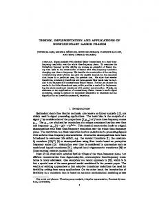
Fig. 1 A computational flow chart for performing the principal component analysis (PCA). The circles identify the input before and after data preprocessing - the raw scans and the difference images - and the outputs: subject loadings and principal components. (A) Data Acquisition: Each of the M subjects gives images aquired under two conditions (e.g., both rest and stimulation conditions). (B) Image Processing: The images are registered and stereotaxically normalized using the method of Friston et al. [20],[21]. Images are then smoothed as desired and gray matter voxels are identified after applying two thresholds. An index of the location of voxels identified as gray matter is derived. Global CBF for each of the unsmoothed images is estimated as the mean of the gray matter voxels. Each of the unsmoothed images are proportionally scaled by dividing each voxel by it’s estimated global CBF. The proportionally scaled unsmoothed images from each of the two conditions are subtracted from one another, i.e., a stimulation minus rest, difference images are derived. (C) Permutation Tests: N permuted versions of the proportionally scaled unsmoothed unthresholded images are derived by randomly permuting the signs of the voxels N times. The permuted and unpermuted versions of the data are then smoothed as desired. The index is then applied to the smoothed images in order to threshold out non-gray matter voxels. The singular values of all the smoothed thresholded data sets are extracted in order to compute the total proportion of variances for each of the extracted components. The variances extracted from the first components extracted from the N permuted data sets are compared to the variance for the first component extracted from the unpermuted data set in order to determine significance. If the variance of the first component extracted is significant, significant tests of the residual variances after each additional component extraction are sequentially tested until one is found to be nonsignificant. The number of components already extracted would then be designated as the number to retain. On the other hand, if the variance of the first component extracted is found to be nonsignificant, the process stops since that would indicate that there is no significant variance in the data. (D) Analytic Rotation of PCs: After the number of components to retain is determined, the reduced set of components extracted from the smoothed, thresholded unpermuted data set are rotated using Harris and Kaiser’s generalization of varimax [17] with Kaiser normalization [15] at the desired level of obliqueness (see Theory).
17
A
Acquire Images
B
Register & Normalize Images
Smooth Images
Derive Index of Gray Matter Voxels
Proportionally Scale Unsmoothed Images
Derive Difference M atrix
Create N Permuted Versions of Difference Matrix
C
Smooth All Data Sets
Select Gray Matter Voxels
Compute PC Variances
Calculate Probability of PC1
NO
Stop
Significant ?
YES
Compute Residual Variance
Calculate Probability of Residual Variance
D
If Number of Significant PCs > 1, Rotate PCs and Subject Loadings
NO
Rotated PCs and Subject Loadings
18
Significant ?
YES
Fig. 2 A plot of the percent of variances for the first components extracted and the percent of residual variances for each subsequent component extracted from the 999 permuted data sets (red) and the unpermuted data set (yellow) for each of the two levels of smoothing (FWHM values of: (a) 20 × 20 × 12 mm and (b) 10 × 10 × 6 mm). The maximum number of components were extracted in order to study the curves of variance values across successive component extractions. The percent of variance values increase to 100 % since after the first component, the percent values represent the percent of the variance left over after the variance of the preceding component(s) have been removed. Comparison of Figures 2 (a) and (b) show three main differences: (1) The number of components found to be significant increased as a function of filter size; (2) Variability of the variance values of the permuted data sets at each component level increased as a function of filter size; and (3) The magnitude of the variance values for the first few components extracted from both the permuted and unpermuted data sets increased as a function of filter size.
19
Fig. 3 In order to evaluate the finding reported in Figures 2(a) and (b), the random permutation test was applied to a synthetic random data set. Figure 3 is a plot of the variance curves extracted from the 999 permuted data sets (red) and the unpermuted data set (yellow) for each of the two levels of smoothing (FWHM values of: (a) 20 × 20 × 12 mm and (b) 10 × 10 × 6 mm). As observed in Figure 2, flucuations in the variance values of the 999 permuted data sets increased as a function of filter size. Also, the magnitude of the percent of variance values extracted from all the data sets (including the unpermuted) increased as a function of filter size. It is worth mentioning that the no significant components were oberseved since by virtue of the data no structure exists. The curve extracted from the unpermuted data set did not markedly differ from the curves extracted from the permuted data sets.
20
Fig. 4 Brain maps illustrating the positive (a) and negative (b) voxel loadings for each of the five obliquely rotated components extracted from the narrative-rest contrast. The loadings are displayed on a standardized MRI scan using methods outlined in the text. Planes of selection from left to right for PC1 are located at -16, +13, +24, +31 and +44 mm; for PC2 are -16, -8, +13, +29, and +37 mm; for PC3 are -5, +3, +11, +29 and 43 mm; for PC4 are -3, +8, +19, +27, and +40 mm; and for PC5 are -8, 0, +8, +29, and +37 mm relative to the anterior commissural-posterior commissural line. The voxel loadings were thresholded at 25 % of the maximum and minmum values for each component. The range of the voxel loadings is coded in the color table. The maximum positive loadings for PC1 to PC5 are 0.442, 0.315, 0.228, and 0.183, respectively. The minumum loadings for PC1 to PC5 are -0.336, -0.316, -0.259, -0.300 and -0.358, respectively. Each of the five components accounted for 21.45, 10.66, 8.77, 8.32 and 17.33 % of the total variance, respectively, accounting for a total of 66.53 %.
21
Fig. 5 Figure 5a is plot of the subject loadings for the first and second unrotated components extracted from the 20 × 20 × 12 mm smoothed data set. The first and second unrotated components accounted for 37.73 and 10.05 percent of the total variance, respectively. The plot suggests no outliers in the data set. Figure 5b shows the plot of the subject loadings for the first and fifth obliquely rotated components extracted from the 20 × 20 × 12 mm smoothed data set. The data represent 11 males and 8 females. Male and female subjects are represented by a different symbols: males, triangle; females, square. The first and fifth obliquely rotated components accounted for 21.45 and 17.33 percent of the total variance, respectively. The plot illustrates how the obliquely rotated components can be useful in identifying clusters or "types" of individuals.
22
Table 1. Corrlelations between the unrotated components extracted after smoothing with the smaller (10x10x6) and larger (20x20x12) smoothing kernals.
20x20x12 mm
10x10x6 mm PC1 PC2 PC3 PC4 PC5
PC1 0.898 0.024 0.055 -0.015 0.016
PC2 -0.038 0.763 0.198 0.043 0.182
23
PC3 0.048 0.159 -0.756 0.121 0.005
PC4 -0.018 -0.196 -0.011 -0.118 0.721
PC5 0.026 -0.021 -0.022 -0.478 -0.181
Unrotated
Table 2. Corrlelations between the unrotated and obliquely rotated components extracted from the 20x20x12 mm smoothed data.
PC1 PC2 PC3 PC4 PC5
PC1 0.705 -0.048 -0.264 0.333 0.567
PC2 0.222 0.880 -0.264 0.002 -0.327
Obliquely Rotated PC3 0.216 -0.385 -0.683 -0.427 -0.342
24
PC4 0.241 0.181 0.355 -0.810 0.357
PC5 0.591 -0.208 0.519 0.104 -0.573
Table 3. Corrlelations between the obliquely rotated components.
PC1 PC2 PC3 PC4
PC2 -0.224
PC3 0.117 -0.180
PC4 -0.321 0.006 -0.059
25
PC5 -0.291 -0.367 -0.070 -0.073
Uncentered
Table 4. Corrlelations between the unrotated component before and after centering.
PC1 PC2 PC3 PC4 PC5
PC1 -0.158 0.864 0.250 0.117 -0.060
Centered PC3 0.045 -0.118 -0.395 0.867 -0.090
PC2 -0.033 0.416 -0.813 -0.200 0.079
26
PC4 0.041 -0.175 -0.314 -0.419 -0.504
PC5 0.448 0.118 0.059 0.093 -0.407
Table 5. Anatomical distribution of voxel loadings. * Positive – premotor, fronto-cingulate and primary sensory cortices. Primary sensory [auditory, visual], premotor [operculum (44/45/6),primary motor cortex (4/6), supplementary motor area, cerebellar hemisphere], anterior cingulate cortex (32)/superior frontal gyrus (8/9). Positive - unimodal visual and heteromodal association cortices, paralimbic cortices and midline cerebellum. Unimodal visual association [fusiform, lateral occipital, inferior temporal gyrus]; heteromodal association [anterior middle temporal gyrus, supramarginal gyrus], paralimbic cortices [dorsal anterior cingulate cortex, parahippocampal gyrus & posterior insula]; midline cerebellum. Positive – operculum, insula, anterior temporal, cingulate and subcortical areas. Bilateral frontal operculum (45/44), anterior insula, dorsolateral prefrontal (46), anterior auditory association cortices, anterior cingulate (32/24) subcortical [basal ganglia, thalamus].
PC1 Negative - heteromodal association cortices. Middle temporal gyrus, dorsolateral prefrontal cortex (10), inferior parietal lobule (angular gyrus).
PC2 Negative - prefrontal cortex, operculum. Medial prefrontal cortex (8, 9, 10, 11), left ventral operculum (47).
PC3 Negative - extrastriate cortices. Bilateral occipital cortex.
PC4 Positive – left lateralized perisylvian cortices, superior Negative – right lateralized operculum, insula, prefrontal cortex, sensorimotor cortex. frontocingulate cortices. Right operculum, anterior insula, dorsolateral prefrontal Left >Right perisylvian cortices [posterior superior cortex (8, 9, 10), anterior cingulate cortex (32). temporal gyrus (posterior auditory association cortices), middle temporal gyrus, angular gyrus - constituents of Wernicke's area]; Left superior frontal gyrus (8, 9, 10); Left > Right primary motor, somatosensory cortex. PC5 Positive - subcortical, opercular, cingulate. Negative – prefrontal, insula, inferior parietal. Subcortical [brainstem, basal ganglia, thalamus]; left Right insula, dorsolateral prefrontal (9, 10). Bilateral ventral operculum (47), dorsal anterior cingulate cortex. angular gyri. * Brodmann areas in parenthesis.
27