Geosci. Model Dev., 2, 89–96, 2009 www.geosci-model-dev.net/2/89/2009/ © Author(s) 2009. This work is distributed under the Creative Commons Attribution 3.0 License.
Geoscientific Model Development
Implementation and evaluation of an array of chemical solvers in the Global Chemical Transport Model GEOS-Chem P. Eller1 , K. Singh1 , A. Sandu1 , K. Bowman2 , D. K. Henze3 , and M. Lee2 1 Department
of Computer Science, Virginia Polytechnic Institute and State University, Blacksburg, VA 24060, USA Jet Propulsion Laboratory, 4800 Oak Grove Drive, Pasadena, CA 91109, USA 3 Earth Institute, Columbia University, 2880 Broadway, New York, NY 10025, USA 2 NASA
Received: 24 October 2008 – Published in Geosci. Model Dev. Discuss.: 5 March 2009 Revised: 5 May 2009 – Accepted: 5 June 2009 – Published: 22 July 2009
Abstract. This paper discusses the implementation and performance of an array of gas-phase chemistry solvers for the state-of-the-science GEOS-Chem global chemical transport model. The implementation is based on the Kinetic PreProcessor (KPP). Two perl parsers automatically generate the needed interfaces between GEOS-Chem and KPP, and allow access to the chemical simulation code without any additional programming effort. This work illustrates the potential of KPP to positively impact global chemical transport modeling by providing additional functionality as follows. (1) The user can select a highly efficient numerical integration method from an array of solvers available in the KPP library. (2) KPP offers a wide variety of user options for studies that involve changing the chemical mechanism (e.g., a set of additional reactions is automatically translated into efficient code and incorporated into a modified global model). (3) This work provides access to tangent linear, continuous adjoint, and discrete adjoint chemical models, with applications to sensitivity analysis and data assimilation.
1
Introduction
GEOS-Chem (http://www-as.harvard.edu/chemistry/trop/ geos/index.html) is a state-of-the-science global 3-D model of atmospheric composition driven by assimilated meteorological observations from the Goddard Earth Observing System (GEOS) of the NASA Global Modeling Assimilation Office (GMAO). GEOS-Chem is used by the atmospheric research community for activities such as assessing intercontinental transport of polluCorrespondence to: A. Sandu
[email protected]
tion, evaluating consequences of regulations and climate change on air quality, comparison of model estimates to satellite observations and field measurements, and fundamental investigations of tropospheric chemistry (http: //www-as.harvard.edu/chemistry/trop/geos/geos pub.html). KPP was originally interfaced with GEOS-Chem and its adjoint in Henze et al. (2007), see Appendices therein. Here we improve upon this implementation in terms of automation, performance, benchmarking, and documentation. The GEOS-Chem native chemistry solver is the Sparse Matrix Vectorized GEAR II (SMVGEARII) code which implements backward differentiation formulas and efficiently solves first-order ordinary differential equations with initial value boundary conditions in large grid-domains (Jacobson and Turco, 1994; Jacobson, 1998). These sparse matrix operations reduce the CPU time associated with LUdecomposition and make the solver very efficient. This code vectorizes all loops about the grid-cell dimension and divides the domain into blocks of grid-cells and vectorizes around these blocks to achieve at least 90% vectorization potential. SMVGEARII uses reordering of grid cells prior to each time interval to group cells with stiff equation together and nonstiff equations together. This allows SMVGEARII to solve equations both quickly and with a high order of accuracy in multiple grid-cell models. Calculation of tropospheric chemistry constitutes a significant fraction of the computational expense of GEOS-Chem. Given the push for running GEOS-Chem at progressively finer resolutions, there is a continual need for efficient implementation of sophisticated numerical methods. This requires a seamless, automated implementation for the wide range of users in the GEOS-Chem community. We present an implementation of GEOS-Chem version 704-10 gas-phase chemistry using the Kinetic PreProcessor KPP. This work extends the set of chemical solvers available
Published by Copernicus Publications on behalf of the European Geosciences Union.
90
P. Eller et al.: Chemical Solvers in the GEOS-Chem CTM
Fig. 1. Flow diagram of implementing GEOS-Chem chemistry with KPP.
to GEOS-Chem users, and provides implementations of tangent linear and adjoint chemical models which are needed in sensitivity analyses and data assimilation studies. The paper is organized as follows. Section 2 briefly reviews KPP capabilities. Section 3 describes the integration of the KPP tools in the GEOS-Chem framework. We discuss the use of two perl parsers (geos2kpp parser.pl, gckpp parser.pl) to modify GEOS-Chem to use a KPP model for gas-phase chemistry. Section 4 presents results demonstrating the effectiveness of this implementation and Sect. 5 draws conclusions and points to future work.
2
The Kinetic PreProcessor KPP
The Kinetic PreProcessor KPP (http://people.cs.vt.edu/ is a software tool to assist computer simulations of chemical kinetic systems (Damian et al., 2002; Sandu and Sander, 2006). The concentrations of a chemical system evolve in time according to the differential law of mass action kinetics. A computer simulation requires an implementation of the differential law and a numerical integration scheme. KPP provides a simple natural language to describe the chemical mechanism and uses a preprocessing step to parse the chemical equations and generate efficient output code in a high level language such as Fortran90, C, or Matlab. A modular design allows rapid prototyping of new chemical kinetic schemes and new numerical integration
∼asandu/Software/Kpp)
Geosci. Model Dev., 2, 89–96, 2009
methods. KPP is being widely used in atmospheric chemistry modeling (Kerkweg et al., 2007; Hakami et al., 2007; Carmichael et al., 2008; Errera and Ronteyn, 2001; Errera et al., 2008; Henze et al., 2007; Henze et al., 2008). The simulation code can be easily re-generated following changes to the chemical mechanism. KPP–2.2 is distributed under the provisions of the GNU license (http://www.gnu.org/copyleft/ gpl.html) and the source code and documentation are available at http://people.cs.vt.edu/∼asandu/Software/Kpp. KPP incorporates a comprehensive library of stiff numerical integrators that includes Rosenbrock, fully implicit Runge-Kutta, and singly diagonally implicit Runge-Kutta methods (Sandu et al., 1997). These numerical schemes are selected to be very efficient in the low to medium accuracy regime. Users can select the method of choice and tune integration parameters (e.g., relative and absolute tolerances, maximal step size) via the optional input parameter vectors ICNTRL U and RCNTRL U. High computational efficiency is attained through fully exploiting sparsity. KPP computes analytically the sparsity patterns of the Jacobian and Hessian of the chemical ODE function, and outputs code that implements the sparse data structures. In this work we make the suite of KPP stiff solvers and the sparse linear algebra routines available in GEOS-Chem. KPP provides tangent linear, continuous adjoint, and discrete adjoint integrators, which are needed in sensitivity analysis and data assimilation studies (Daescu et al., 2003; Sandu et al, 2003). Flexible direct-decoupled and adjoint sensitivity code implementations are achieved with minimal user intervention. The resulting sensitivity code is highly efficient, taking full advantage of the sparsity of the chemical Jacobians and Hessians. Adjoint modeling is an efficient tool to evaluate the sensitivity of a scalar response function with respect to the initial conditions and model parameters. 4D-Var data assimilation allows the optimal combination of a background estimate of the state of the atmosphere, knowledge of the interrelationships among the chemical fields simulated by the model, and observations of some of the state variables. An optimal state estimate is obtained by minimizing an objective function to provide the best fit to all observational data (Carmichael et al., 2008). Three dimensional chemical transport models whose adjoints have been implemented using KPP include STEM (Carmichael et al., 2008), CMAQ (Hakami et al., 2008), BASCOE (Errera et al. 2008; Errera et al. 2001), and an earlier version of GEOS-Chem (Henze et al., 2007; Henze et al., 2008).
3
Implementation of GEOS-Chem with KPP
In this section we discuss the incorporation of the KPP generated gas-phase chemistry simulation code in GEOS-Chem. A simple three step process modifies GEOS-Chem version 7-04-10 to use KPP. This process is summarized in Fig. 1. First, the geos2kpp parser.pl reads the chemical mechanism www.geosci-model-dev.net/2/89/2009/
P. Eller et al.: Chemical Solvers in the GEOS-Chem CTM description file globchem.dat and creates three KPP input files – also containing information on the chemical mechanism, but in KPP format. Second, KPP processes these input files and generates Fortran90 chemical simulation code; the model files are then copied into the GEOS-Chem v704-10 directory. A special directive has been implemented in KPP to generate code that interfaces with GEOS-Chem. The third step involves running the gckpp parser.pl to modify GEOS-Chem source code to correctly call the KPP generated gas-phase chemistry simulation routines. The process is discussed in detail below. 3.1
Automatic translation of SMVGEARII inputs to KPP inputs using geos2kpp parser.pl
KPP requires a description of the chemical mechanism in terms of chemical species (specified in the *.spc file), chemical equations (specified in the *.eqn file), and mechanism definition (specified in the *.def file). The syntax of these files is specific, but simple and intuitive for the user. Based on this input KPP generates all the Fortran90 (or C/Matlab) files required to carry out the numerical integration of the mechanism with the numerical solver of choice. GEOS-Chem SMVGEARII uses the mechanism information specified in the “globchem.dat” file; this file contains a chemical species list and a chemical reactions list. The perl parser geos2kpp parser.pl translates the chemical mechanism information from “globchem.dat” into the KPP syntax and outputs it in the files “globchem.def”, “globchem.eqn”, and “globchem.spc”. The globchem.dat chemical species list describes each species by their name, state, default background concentration, and additional characteristics. For example, consider the description of the following two species in the SMVGEARII syntax globchem.dat: A A3O2 1.00 1.000E-20 1.000E-20 1.000E-20 1.000E-20 I ACET 1.00 1.000E-20 1.000E-20 1.000E-20 1.000E-20
91 globchem.spc: #DEFVAR A302 = IGNORE; #DEFFIX ACET = IGNORE; globchem.def: A3O2 = 1.000E-20; ACET = 1.000E-20; The globchem.dat chemical reactions list describes each reaction by their reactants, products, rate coefficients, and additional characteristics. This information is processed by geos2kpp parser.pl to create the “globchem.eqn” file, which contains the chemical equation information in KPP format. KPP uses GEOS-Chem’s calculated rate constants instead of using the kinetic parameters listed next to each chemical equation. A comparison of “globchem.dat” and “globchem.eqn” is shown below. globchem.dat: A 21 3.00E-12 0.0E+00 -1500 0 0.00 0 0 O3 + NO =1.000NO2 + 1.000O2 globchem.eqn: {1} O3 + NO = NO2 + O2 : ARR(3.00E-12, 0.0E00, -1500.0); The perl parser geos2kpp parser.pl makes the translation of the chemical mechanism information a completely automatic process. The user has to invoke the parser with the “globchem.dat” input file and obtains the KPP input files. The use of the perl parser is illustrated below: [user@local ] $ perl -w geos2kpp parser.pl globchem.dat Parsing globchem.dat Creating globchem.def, globchem.eqn, and globchem.spc
1
This information is parsed by geos2kpp parser.pl and translated automatically into the KPP syntax. Specifically, the species are defined in the “globchem.spc” file and are declared as variable (A, active) or fixed (I, inactive). Variable refers to medium or short lived species whose concentrations vary in time and fixed refers to species whose concentrations do not vary too much. Species are set equal to the predefined atom IGNORE to avoid doing a species mass-balance checking for the GEOS-Chem implementation of KPP. The default initial concentrations are written in the file “globchem.def” as shown below.
3.2
Creation of KPP model to interface with GEOSChem
Once the input files are ready, KPP is called to generate all Fortran90 subroutines needed to describe and numerically integrate the chemical mechanism. We have slightly modified the KPP code generation engine to assist the integration of the KPP subroutines within GEOS-Chem. A new KPP input command (#GEOSCHEM) instructs to produce code that can interface with GEOS-Chem. This command is added to the KPP input file *.kpp, along with specifying details such as the name of the model created in the first step and integrator to use. A sample *.kpp file is shown below.
1 The last four values represent the default volume mix ratio in the stratosphere, troposphere(land and sea), and urban regions.
www.geosci-model-dev.net/2/89/2009/
Geosci. Model Dev., 2, 89–96, 2009
92
P. Eller et al.: Chemical Solvers in the GEOS-Chem CTM
gckpp.kpp: #MODEL globchem #INTEGRATOR rosenbrock #LANGUAGE Fortran90 #DRIVER none #GEOSCHEM on
Modifying gckpp Integrator.f90 ... Modifying chemistry mod.f Creating Makefile.ifort.4d ... Creating checkpoint mod.f Done modifying GEOS-Chem files
KPP is invoked with this input file [user@local ] $ kpp gckpp.kpp and generates complete code to perform forward and adjoint chemistry calculations. The model files are named gckpp * or gckpp adj *, respectively. These files are then copied into the GEOS-Chem code directory. 3.3
Automatic modification of GEOS-Chem source code to interface with KPP chemistry routines using gckpp parser.pl
The last step involves running the gckpp parser.pl to modify the GEOS-Chem source code to interface with KPP. This parser is run once in the GEOS-Chem code directory, modifies existing files to use KPP instead of SMVGEARII for the chemistry step, and adds new files with subroutines for adjoint calculations. The GEOS-Chem code modifications are necessary for a correct data transfer to and from KPP. The chemical species concentrations are mapped between GEOS-Chem and KPP at the beginning of each timestep. This is done through copying data from the three-dimensional GEOS-Chem data structures to the KPP data structures for each grid cell. At the end of the time step the time-evolved chemical concentrations are copied from KPP back into GEOS-Chem. Since KPP performs a reordering of the chemical species to enhance sparsity gains, the species indices are different in KPP than in GEOS-Chem. The KPP-generated “kpp Util.f90” file provides the subroutines Shuffle user2kpp and Shuffle kpp2user which maps a user provided array to a KPP array and viceversa. These subroutines are used to initialize the VAR and FIX species of KPP with the CSPEC array values from SMVGEARII (for each grid cell JLOOP). GEOS-Chem calculates the reaction rates for each equation in each grid cell at the beginning of each chemistry step. These rate coefficients are mapped from the SMVGEARII reaction ordering to the KPP ordering via a reshuffling, and are saved. Prior to each call to the KPP integrator, the reaction rates for the particular grid cell are copied from the storage matrix into the local KPP integration data structures. The use of the gckpp parser.pl perl parser is illustrated below. The parser outputs a message for each modified or created file. [user@local ] $ perl -w gckpp parser.pl Modifying and creating GEOS-Chem files Geosci. Model Dev., 2, 89–96, 2009
The resulting GEOS-Chem code now uses KPP for gasphase chemistry. Makefiles are included for the finitedifference driver, sensitivity driver, and 4D-Var driver.
4
Evaluation of GEOS-Chem with KPP
We evaluate GEOS-Chem using global chemistry-only simulations. GEOS-Chem models a wide variety of chemical regimes including urban and rural, tropospheric and stratospheric, and day and night during each simulation. We use 106 chemical species (87 variables species and 19 fixed species), 311 reactions, and 43858 grid cells. This requires about 35MB of data to hold species concentrations and 104MB of data to hold the reaction rates. Experiments are performed on an 8-core Intel Xeon E5320 @ 1.86 GHz. Additional details on the test machine are included in the appendix. This is a typical configuration for a small shared memory machine. In order to illustrate the correctness of GEOS-Chem simulations using KPP for gas-phase chemistry we compare the results against the original simulation with SMVGEARII. GEOS-Chem is run for 48 h from 00:00 GMT on 1 July 2001 to 23:00 GMT on 2 July 2001. One simulation uses SMVGEARII chemistry and the second uses the KPP chemical code; the simulations are identical otherwise. Concentrations are checkpointed every hour and then compared. Plots of Ox concentrations (O3+O1D+O3P) at the end of the 48 h simulation are presented in Fig. 2a. Both simulations produce visually identical results. A difference plot is presented in Fig. 2b which shows less than 1% error between the SMVGEARII computed concentrations and KPP computed concentrations. A more stringent validation is provided by the scatter plot of SMVGEARII vs KPP/Rodas3 results. The simulation interval is one week, between 00:00 GMT on 1 July 2001 and 23:00 GMT on 7 July 2001, using an absolute tolerance of ATOL=10−1 and a relative tolerance of RTOL=10−3 . Both simulations are started with the same initial conditions and they differ only in the chemistry module. The results are shown in Fig. 3. Each point in the scatter plot corresponds to the final Ox concentration in a different grid cell. The Ox concentrations obtained with KPP and with SMVGEARII are very similar to each other. We compare the computed concentrations of the SMVGEARII and KPP solvers against a reference solution for each solver. Solutions are calculated using www.geosci-model-dev.net/2/89/2009/
P. Eller et al.: Chemical Solvers in the GEOS-Chem CTM
93
Fig. 3. Scatterplot of Ox concentrations (molecules/cm3 ) computed with SMVGEARII and KPP for a one week simulation (Mean Error=0.05%, Median Error=0.03%).
Fig. 2. (a) SMVGEARII and KPP/Rodas3 computed Ox concentrations (Parts per billion volume ratio) for a 48 h simulation (b) Difference between SMVGEARII and KPP/Rodas3 computed Ox concentrations.
relative tolerances (RTOL) in the range 10−1 ≤RTOL≤10−3 and absolute tolerances ATOL=104 ×RTOL molecules cm−3 . Reference solutions are calculated using RTOL=10−8 and ATOL=10−3 molecules cm−3 . Following Henze et al. (2007) and Sandu et al. (1997), we use significant digits of accuracy(SDA) to measure the numerical errors. We calculate SDA using ref 2 !−1 X X ck,j −b ck,j SDA = − log10 max 1 · ref k ck,j c ≥a c k,j
k,j ≥a
This uses a modified root mean square norm of the relative error of the solution (b ck,j ) with respect to the reference soref ) for species k in grid cell j . A threshold value lution (ck,j of a=106 molecules cm−3 avoids inclusion of errors from species concentrations with very small values. Figure 4 presents a work-precision diagram where the number of accurate digits in the solution is plotted against the time needed by each solver to integrate the chemical mechanism. A seven day chemistry-only simulation from 00:00 GMT on 1 July 2001 to 00:00 GMT on 8 July 2001 is completed using the KPP Rosenbrock Rodas3, Rosenbrock Rodas4, Runge-Kutta, and Sdirk integrators and with www.geosci-model-dev.net/2/89/2009/
the SMVGEARII integrator for each tolerance level. The results indicate that, for the same computational time, the KPP Rosenbrock integrators produce a more accurate solution than the SMVGEARII integrator. The Sdirk and RungeKutta integrators are slower at lower tolerances as shown in Fig. 4 in comparison to the Rosenbrock and SMVGEARII integrators. The Runge-Kutta and Sdirk integrators normally take longer steps, but they take fewer steps at higher tolerances. Since we normally use tolerances of 10−3 or lower for GEOS-Chem, we do not get these advantages. These results are similar to the results produced by Henze et al. (2007) through demonstrating that the KPP Rosenbrock solvers are about twice as efficient as SMVGEARII for a moderate level of accuracy. Note that none of the KPP solvers uses vectorization. In addition to the solvers discussed above we have also tested LSODE (Radakrishan and Hindmarsh, 1993), modified to use the KPP generated sparse linear algebra routines. LSODE is based on the same underlying mathematical formulas as SMVGEARII. The LSODE solution provides 3–4 accurate digits for a computational time of about 300 s (this would place LSODE in the upper left corner of Fig. 4). Since LSODE does not reach the asymptotic regime for the low accuracy tolerances used here we do not report its results further. Table 1 compares the reference solutions obtained with SMVGEARII, Rodas3, Rodas4, Runge-Kutta, and Sdirk integrators through showing the number of significant digits of accuracy produced when comparing two integrators. The results show that Rodas3, Rodas4, and Sdirk produce very similar references, while the SMVGEARII and Runge-Kutta solutions have between 0.5 and 4.0 digits of accuracy for each chemical species when compared to other integrators. The GEOS-Chem/KPP parallel code is based on OpenMP and uses THREADPRIVATE variables to allow multiple Geosci. Model Dev., 2, 89–96, 2009
94
P. Eller et al.: Chemical Solvers in the GEOS-Chem CTM
Integrator Rodas3–SMVGEARII Rodas3–Rodas4 Rodas3–Runge-Kutta Rodas3–Sdirk Rodas4–SMVGEARII Runge-Kutta–SMVGEARII Sdirk–SMVGEARII
Significant Digits of Accuracy
3
2.5
NOx
Ox
PAN
CO
2.1 8.3 2.1 8.5 2.1 2.6 2.1
3.3 9.8 3.3 9.5 3.3 3.8 3.3
0.5 7.6 2.7 7.8 0.5 0.5 0.5
3.7 10.4 4.0 10.2 3.7 3.0 3.7
Rosenbrock Rodas3 Rosenbrock Rodas4 Runge−Kutta SDIRK SMVGEAR
2
Table 2. Comparison of the average number of function calls and chemical time steps per advection time step per grid cell. Integrator Rodas3 Rodas4 Runge-Kutta Sdirk SMVGEARII
CPU Time on 1 Processor/CPU Time on P Processors
Table 1. Direct comparison of the number of significant digits of accuracy produced by Rodas3, Rodas4, Runge-Kutta, Sdirk, and SMVGEAR reference solutions for NOx , Ox , PAN, and CO for a one week chemistry-only simulation.
1.5
8
7
Function Calls
Steps
9 18 22 27 39
3 3 2 2 28
Rosenbrock RODAS3 Rosenbrock RODAS4 SMVGEAR Runge−Kutta SDIRK
6
5
4
3
2
1 1
2
3
4 5 Number of Processors
6
7
8
1
200
400
Time (sec)
800
1600
Fig. 4. Work-precision diagram (Significant Digits of Accuracy for Ox versus run time) for a seven day chemistry-only simulation for RTOL=1.0E-1, 3.0E-2, 1.0E-2, 3.0E-3, 1.0E-3 (lower left to upper right). Rodas4 does not have a point for RTOL=1.0E-1 due to not producing meaningful results.
threads to concurrently execute the KPP chemistry for different grid cells. To illustrate the impact of the new chemistry code on parallel performance we consider a sevenday chemistry-only simulation from 00:00 GMT on 1 July 2001 to 00:00 GMT on 8 July 2001 using a relative tolerance of 3×10⁻² and an absolute tolerance of 10−2 molecules/cm3 and employ 1, 2, 4, and 8 processors. Figure 5 illustrates the parallel speedups for the KPP Rodas3 and Rodas4 integrators and for SMVGEARII; the code has close to linear speedups for all integrators. Table 2 compares the average number of function calls made and average number of steps taken by each integrator per advection time step per grid cell. These results correlate well with those in Fig. 4: the KPP integrators performing fewer function calls are faster. A novel capability offered by the KPP chemistry is a readily available adjoint chemical model. Adjoint models are the essential computational ingredient for sensitivity analyses and for 4D-Var data assimilation. As an illustration of adjoint sensitivity analysis with GEOS-Chem we consider a Geosci. Model Dev., 2, 89–96, 2009
Fig. 5. Speedup plot for Rosenbrock Rodas3, Rosenbrock Rodas4, SMVGEARII, Runge-Kutta, and Sdirk for a 7 day chemistry-only simulation.
possible TES (Tropospheric Emission Spectrometer) trajectory (illustrated in Fig. 6) and assume that a measurement of the total ozone column underneath the trajectory is taken at 1st April 2001. The TES trajectory contains the latitude and longitude coordinates of the trajectory of the satelite position in time. We use adjoint sensitivity analysis to assess how this measurement carries information about total NOx emissions in the week preceding April 1st, 2001. Specifically, we calculate scaled adjoint sensitivities of the ozone column with respect to total NOx emissions; the distribution of these sensitivities illustrated in Fig. 6 demonstrates the sensitivity of O3 over the TES trajectory with respect to the NOx emissions. See Henze et al. (2007) for a more detailed discussion of the adjoint of GEOS-Chem.
5
Conclusions
The widely used state-of-the-science GEOS-Chem model has been added the capability of using KPP to build the gasphase chemistry simulation code. The GEOS-Chem/KPP interface is automatic and requires no additional programming effort. The geos2kpp parser.pl converts the GEOSChem input files to KPP input files, while gckpp parser.pl modifies GEOS-Chem to interface with KPP. Updates to KPP assist the model integration. These tools provide the www.geosci-model-dev.net/2/89/2009/
P. Eller et al.: Chemical Solvers in the GEOS-Chem CTM
95 References
Fig. 6. Sensitivity of the O3 column measured by TES with respect to the NOx emissions (parts per billion volume) over Asia on 1st April 2001.
global chemical transport modeling community with access to highly efficient solvers, a wide variety of user options, and access to tangent linear, continuous adjoint, and discrete adjoint chemical models. Our results demonstrate that the KPP solvers and the native GEOS-Chem solver (SMVGEARII) produce accurate results as demonstrated through visual examination as well as difference plots. The KPP Rodas3 and Rodas4 solvers achieve a similar level of accuracy at a lower computational expense than the SMVGEARII solver as demonstrated through the SDA plot. Additionally the tested KPP solvers have comparable scalability for parallel processing as the SMVGEARII solver.
Appendix A Test Setup System: 8-core Intel Xeon x86 64 E5320 @ 1.86 GHz RAM: 8192MB Cache: 4096KB per core Operating System: Fedora Core 8, Kernel 2.6.26.8 Compiler: Intel Fortran Compiler fce 10.1.008 Compiler Options: -cpp -w -O2 -auto -noalign -convert big endian -openmp -Dmultitask
Acknowledgements. This work was supported by NASA through the ROSES-2005 AIST award. Edited by: P. Joeckel
www.geosci-model-dev.net/2/89/2009/
Carmichael, G. R., Chai, T., Sandu, A., Constantinescu, E. M., and Daescu, D.: Predicting Air Quality Improvements through Advanced Methods to Integrate Models and Measurements, J. Comp. Phys., 227, 3540–3571, 2008. Daescu, D., Sandu, A., and Carmichael, G. R.: Direct and Adjoint Sensitivity Analysis of Chemical Kinetic Systems with KPP: II – Validation and Numerical Experiments, Atmos. Environ., 37, 5097–5114, 2003. Damian, V., Sandu, A., Damian, M., Potra, F., and Carmichael, G. R.: The Kinetic PreProcessor KPP - A Software Environment for Solving Chemical Kinetics, Comp. and Chem. Eng., 26(11), 1567–1579, 2002. Errera, Q., Daerden, F., Chabrillat, S., Lambert, J. C., Lahoz, W. A., Viscardy, S., Bonjean, S., and Fonteyn, D.: 4D-Var assimilation of MIPAS chemical observations: ozone and nitrogen dioxide analyses, Atmos. Chem. Phys., 8, 6169–6187, 2008, http://www.atmos-chem-phys.net/8/6169/2008/. Errera, Q. and Fonteyn, D: Four-dimensional variational chemical assimilation of CRISTA stratospheric measurements, J. Geos. Phys., 106(D11), 12253–12265, 2001. Hakami, A., Henze, D. K., Seinfeld, J. H., Singh, K., Sandu, A., Kim, S., Byun, D., and Li, Q.: The Adjoint of CMAQ, Environ. Sci. Technol., 41(22), 7807–7817, 2007. Henze, D. K., Hakami, A., and Seinfeld, J. H.: Development of the Adjoint of GEOS-Chem, Atmos. Chem. Phys., 7, 2413–2433, 2007, http://www.atmos-chem-phys.net/7/2413/2007/. Henze, D. K., Seinfeld, J. H., Ng, N. L., Kroll, J. H., Fu, T.-M., Jacob, D. J., and Heald, C. L.: Global modeling of secondary organic aerosol formation from aromatic hydrocarbons: high- vs. low-yield pathways, Atmos. Chem. Phys., 8, 2405–2420, 2008, http://www.atmos-chem-phys.net/8/2405/2008/. Jacobson, M. Z.: Technical Note: Improvement of SMVGEAR II on Vector and Scalar Machines through Absolute Error Tolerance Control, Atmos. Environ., 32, 791–796, 1998. Jacobson, M. Z. and Turco, R.: SMVGEAR: A Sparse-Matrix, Vectorized Gear Code For Atmospheric Models, Atmos. Environ., 28, 273–284, 1994. Kerkweg, A., Sander, R., Tost, H., Jockel, P., and Lelieveld, J.: Technical Note: Simulation of Detailed Aerosol Chemistry on the Global Scale using MECCA-AERO, Atmos. Chem. Phys., 7, 2973–2985, 2007, http://www.atmos-chemphys.net/7/2973/2007/. Radhakrishnan, K. and Hindmarsh, A. C.: Description and Use of LSODE, the Livermore Solver for Ordinary Differential Equations, LLNL report UCRL-ID-113855, December 1993. Sandu, A., Daescu, D., and Carmichael, G. R.: Direct and Adjoint Sensitivity Analysis of Chemical Kinetic Systems with KPP: I – Theory and Software Tools, Atmos. Environ., 37, 5083–5096, 2003. Sandu, A. and Sander, R.: Technical Note: Simulating Chemical Kintetic Systems in Fortran90 and Matlab with the Kinetic PreProcessor KPP-2.1, Atmos. Chem. Phys., 6, 1–9, 2006, http://www.atmos-chem-phys.net/6/1/2006/. Sandu, A., Verwer, J. G., Blom, J. G., Spee, E. J., Carmichael, G. R., and Potra, F. A.: Benchmarking stiff ODE solvers for atmospheric chemistry problems I: Implicit versus Explicit, Atmos. Environ., 31, 3151–3166, 1997a.
Geosci. Model Dev., 2, 89–96, 2009
96
P. Eller et al.: Chemical Solvers in the GEOS-Chem CTM
Sandu, A., Verwer, J. G., Blom, J. G., Spee, E. J., Carmichael, G. R., and Potra, F. A.: Benchmarking stiff ODE solvers for atmospheric chemistry problems II: Rosenbrock methods, Atmos. Environ., 31, 3459–3472, 1997b.
Geosci. Model Dev., 2, 89–96, 2009
www.geosci-model-dev.net/2/89/2009/