Development and evaluation of an Earth-System ... - Geosci. Model Dev.

Geosci. Model Dev., 4, 1051–1075, 2011 www.geosci-model-dev.net/4/1051/2011/ doi:10.5194/gmd-4-1051-2011 © Author(s) 2011. CC Attribution 3.0 License.

Geoscientific Model Development

Development and evaluation of an Earth-System model – HadGEM2 W. J. Collins1 , N. Bellouin1 , M. Doutriaux-Boucher1 , N. Gedney1 , P. Halloran1 , T. Hinton1 , J. Hughes1 , C. D. Jones1 , M. Joshi2 , S. Liddicoat1 , G. Martin1 , F. O’Connor1 , J. Rae1 , C. Senior1 , S. Sitch3 , I. Totterdell1 , A. Wiltshire1 , and S. Woodward1 1 Met

Office Hadley Centre, Exeter, UK Centres for Atmospheric Science, Climate Directorate, Dept. of Meteorology, University of Reading, Earley Gate, Reading, UK 3 School of Geography, University of Leeds, Leeds, UK 2 National

Received: 23 March 2011 – Published in Geosci. Model Dev. Discuss.: 13 May 2011 Revised: 9 September 2011 – Accepted: 14 November 2011 – Published: 29 November 2011

Abstract. We describe here the development and evaluation of an Earth system model suitable for centennial-scale climate prediction. The principal new components added to the physical climate model are the terrestrial and ocean ecosystems and gas-phase tropospheric chemistry, along with their coupled interactions. The individual Earth system components are described briefly and the relevant interactions between the components are explained. Because the multiple interactions could lead to unstable feedbacks, we go through a careful process of model spin up to ensure that all components are stable and the interactions balanced. This spun-up configuration is evaluated against observed data for the Earth system components and is generally found to perform very satisfactorily. The reason for the evaluation phase is that the model is to be used for the core climate simulations carried out by the Met Office Hadley Centre for the Coupled Model Intercomparison Project (CMIP5), so it is essential that addition of the extra complexity does not detract substantially from its climate performance. Localised changes in some specific meteorological variables can be identified, but the impacts on the overall simulation of present day climate are slight. This model is proving valuable both for climate predictions, and for investigating the strengths of biogeochemical feedbacks.

Correspondence to: W. J. Collins ([email protected])

1

Introduction

The Hadley Centre Global Environmental Model version 2 (HadGEM2) family of models has been designed for the specific purpose of simulating and understanding the centennial scale evolution of climate including biogeochemical feedbacks. The Earth system configuration is the first in the Met Office Hadley Centre to run without the need for flux corrections. The previous Hadley Centre climate model (HadGEM1) (Johns et al., 2006) did not include biogeochemical feedbacks, and the previous carbon cycle model in the Hadley Centre (HadCM3LC) (Cox et al., 2000) used artificial correction terms to the ocean heat fluxes to keep the model state from drifting. In this paper, we use the term Earth system model to refer to the set of equations describing physical, chemical and biological processes within and between the atmosphere, ocean, cryosphere, and the terrestrial and marine biosphere. We exclude from our definition here any representation of solid Earth processes. There is no strict definition of which processes at what level of complexity are required before a climate model becomes an Earth system model. Many climate models contributing to the CMIP3 project (Meehl et al., 2007) included some Earth system components. For example HadGEM1 (Johns et al., 2006), the predecessor to HadGEM2, already included a land surface scheme and some interactive aerosols; however typically the term “Earth system” is used for those models that at least include terrestrial and ocean carbon cycles. The inclusion of Earth system components in a climate model has a two-fold benefit. It allows a consistent calculation of the impacts of climate change on atmospheric composition or ecosystems for example, which can be scientifically

Published by Copernicus Publications on behalf of the European Geosciences Union.

1052

W. J. Collins et al.: Development and evaluation of an Earth-System model – HadGEM2

valuable in its own right (e.g. Jones et al., 2009). The second benefit is that it allows the incorporation of biogeochemical feedbacks which can be negative, dampening the sensitivity of the climate to external forcing (e.g. Charlson et al., 1987), or positive, amplifying the sensitivity (e.g. Cox et al., 2000). These feedbacks will either affect predictions of future climate for a given forcing, or for a given desired climate outcome (such as limiting warming below 2 K above pre-industrial values) will affect the calculations of allowable emissions (e.g. Jones et al., 2006). Earth system models have the ability to be driven with either concentrations or emissions of greenhouse gases (particularly CO2 ). Adding Earth systems components and processes increases the complexity of the model system. Many biogeochemical processes are less well understood or constrained than their physical counterparts. Hence the model spread in future projections is considerably larger and better represents the true uncertainty of the future evolution of climate. Booth and Jones (2011) found that the spread in predicted temperatures due to uncertainty in just the carbon cycle modelling was comparable to the spread due to uncertainty in all the physical parameters. Many studies to compare models with each other and with measurements have been undertaken (e.g. Eyring et al., 2006; Friedlingstein et al., 2006; Stevenson et al., 2006; Textor et al., 2006; Sitch et al., 2008; Blyth et al., 2011) to identify the uncertainties at the process level. Notwithstanding these uncertainties, neglecting Earth system processes introduces systematic bias. Similarly, Earth system models cannot include every process, due to lack of knowledge or lack of computational power, and so will have an inherent but often unknown bias. For example many models neglect the nitrogen cycle. This cycle may exacerbate climate warming through restricting the ability of vegetation to respond to CO2 fertilisation, or may reduce climate warming through the fertilising effect of anthropogenic emissions of reactive nitrogen compounds. However the role and mechanisms by which the nitrogen cycle modulates the climatecarbon cycle system are currently uncertain. The extra complexity of an Earth system model is needed to understand how the climate may evolve in future, but it is likely to degrade the model’s simulation of the present day climate since driving inputs originally derived from observed quantities (such as vegetation distribution and atmospheric composition) are replaced by interactive schemes that are necessarily imperfect. An analogy can be drawn with the progression from atmosphere-only models which used observed sea surface temperatures (SSTs), to coupled atmosphere-ocean models which do not represent the present day SSTs perfectly, but allow examination of modes of variability and feedbacks. For Earth system models, as with the coupled atmosphere-ocean models, care has to be taken to ensure that the present day simulations are not taken too far from the observed state so that the simulations of the climate evolution are not credible.

Geosci. Model Dev., 4, 1051–1075, 2011

The Met Office Hadley Centre Earth system model was designed to include the biogenic feedbacks thought to be most important on centennial timescales, whilst taking into account the level of scientific understanding and state of model development for the different processes. The level of complexity was also restricted by the need to be able to complete centennial-scale integrations on a reasonable timescale. Thus the focus for HadGEM2 is on terrestrial and ocean ecosystems, gas and aerosol phase composition, and the interactions between these components.

2

Model components

The HadGEM2 Earth system model (HadGEM2-ES) comprises underlying physical atmosphere and ocean components with the addition of schemes to characterise aspects of the Earth system. The particular Earth system components that have been added to create the HadGEM2 Earth system model discussed in this paper are the terrestrial and oceanic ecosystems, and tropospheric chemistry. The ecosystem components TRIFFID (Cox, 2001) and diatHadOCC (Palmer and Totterdell, 2001) are introduced principally to enable the simulation of the carbon cycle and its interactions with the climate. Diat-HadOCC also includes the feedback of dust fertilisation on plankton growth. The UKCA scheme (O’Connor et al., 2009, 2011) is used to model tropospheric chemistry interactively, allowing it to vary with climate. UKCA affects the radiative forcing through simulating changes in methane and ozone, as well as the rate at which sulphur dioxide and DMS emissions are converted to sulphate aerosol. In HadGEM1 the chemistry was provided through climatological distributions that were unaffected by meteorology or climate. Although the HadGEM2 model was designed from the outset to include the above Earth system components, they can be readily de-activated and the data they produce replaced with relevant climatological mean values. A paper (The HadGEM2 Model Development Team, 2011) describes how these components can be combined to create different configurations of HadGEM2 that are in use. Particular configurations from that paper to be noted are HadGEM2-ES which includes all the earth system components to be described here, and HadGEM2-CC which includes the all the earth system components except the gas-phase tropospheric chemistry. We also describe in this paper improvements to components of HadGEM2 which could be considered as part of the Earth system, but are not readily de-activated and therefore still required in the “physics-only” model configuration referred to as HadGEM2-AO. These components are: hydrology, land surface exchange scheme, river routing and aerosols. A list of the Earth system components and couplings is provided in Table 1. The individual components have been calibrated separately and evaluated in the complete Earth system set up. www.geosci-model-dev.net/4/1051/2011/

W. J. Collins et al.: Development and evaluation of an Earth-System model – HadGEM2

1053

Table 1. Summary of main Earth system additions from HadGEM1 to HadGEM2-ES. Earth System components

Reason for inclusion

New Components Terrestrial Carbon cycle

TRIFFID dynamic vegetation scheme (Cox, 2001)

To model the exchange of CO2 between the atmosphere and the terrestrial biosphere, and to model changes in the vegetation distribution.

Ocean carbon cycle

diat-HadOCC ocean biology scheme (Palmer and Totterdell, 2001)

To model the exchange of carbon dioxide between the atmosphere and the oceanic biosphere

Atmospheric Chemistry

UKCA tropospheric chemistry scheme

To allow the ozone and methane radiative forcing fields, and the sulphate oxidant fields to vary with meteorology and climate

Aerosols

Fossil-fuel organic carbon, ammonium nitrate, dust and biogenic organic aerosols added

These important anthropogenic and natural aerosol species are now represented in the model

New couplings

2.1

Chemistry-radiation

Radiative effects of O3 and CH4 are taken from the interactive chemistry

This allows the concentrations of these species to vary with climate and tropopause heights.

Chemistry-hydrology

The emissions of methane from wetlands are supplied from the hydrology scheme to the chemistry scheme.

The emissions and hence concentrations of methane will vary as climate impacts on the extent of wetlands

Chemistry-Aerosols

Sulphate oxidation scheme takes its oxidants from the interactive chemistry.

The sulphur oxidation will now be affected by meteorology and climate

Ocean carbon cycle-DMS

DMS emission now interactively generated by the ocean biology

This important source of sulphate aerosol will now vary as climate change affects the plankton

Vegetation-Dust

Dust emissions depend on the bare soil fraction generated by the vegetation scheme

Dust production will vary as climate change affects the vegetation distribution

Dust-Ocean carbon cycle

Dust deposition affects plankton growth

The supply of nutrients to the plankton varies with the dust production. This coupling also allows geo-engineering experiments to be simulated.

Underlying physical model

The physical model configuration is derived from the HadGEM1 climate model (Johns et al., 2006 and references therein) with improvements as discussed in The HadGEM2 Development Team (2011) and Martin et al. (2010), and is only described briefly here. The atmospheric component uses a horizontal resolution of 1.25◦ × 1.875◦ in latitude and longitude with 38 layers in the vertical extending to over 39 km in height. The oceanic component uses a latitude– longitude grid with a zonal resolution of 1◦ everywhere and meridional resolution of 1◦ between the poles and 30◦ latitude, from which it increases smoothly to 1/3◦ at the equator. It has 40 unevenly spaced levels in the vertical. The addition of Earth system components to the climate model introduces more stringent criteria on the physical perwww.geosci-model-dev.net/4/1051/2011/

formance. For instance, the existence of biases in temperature or precipitation on the regional scale need not detract from a climate model’s ability to simulate future changes in climate; however such biases can seriously affect the ability of the Earth system model to simulate reasonable vegetation distributions in these areas. Hence a focus for the development of the physical components of HadGEM2 was improving the surface climate, as well as other outstanding errors such as El Ni˜no Southern Oscillation (ENSO) and tropical climate. Details of the major developments to the physical basis of the HadGEM2 model family are described in Martin et al. (2010) and The HadGEM2 Development Team (2011). 2.2

Land surface exchange scheme

The land surface scheme in HadGEM2 is MOSES II (Essery et al., 2003), from which the JULES scheme (Best et Geosci. Model Dev., 4, 1051–1075, 2011

1054

W. J. Collins et al.: Development and evaluation of an Earth-System model – HadGEM2

al., 2011; Clark et al., 2011) is derived. This was targeted for development since surface exchange directly influences the vegetation scheme and the terrestrial carbon cycle. Even without land carbon-climate feedbacks, these changes improve the land-surface exchange since water loss through leaves (transpiration) and carbon gain (GPP, gross primary productivity) are intimately linked through the leaf stomatal conductance. There is an improved treatment of penetration of light through the canopy (Mercado et al., 2007). This involves explicit description of light interception for different canopy levels, which consequently allows a multilayer approach to scaling from leaf to canopy level photosynthesis. The multilayer approach has been evaluated against eddy-correlation data at a temperate conifer forest (Jogireddy et al., 2006) and at a tropical broad-leaved rainforest site (Mercado et al., 2007), and these studies demonstrated the improved model performance with the multi-layer approach compared with the standard big-leaf approach. The original MOSES II scheme removed excess water by adding it straight into the surface runoff if the top soil level was saturated. In HadGEM2 this is modified to add this into the downward moisture flux in order to retain soil moisture better (Martin et al., 2010). Lakes in MOSES II do not vary with climate, so the areas remain constant. In HadGEM1 evaporation from lakes was therefore a net source of water into the climate system. In HadGEM2 this evaporation now depletes the soil moisture. It would have been desirable to take this from the surface grid squares containing the lake, but this often led to unacceptably low soil moisture levels. As a compromise, the global lake evaporation flux is calculated and removed evenly from the deep soil moisture over the whole land surface (providing the soil moisture content is greater than the wilting point in the grid box). This water conservation is necessary to diagnose trends in sea level. Precipitation falling onto a grid square adds to the soil moisture regardless of the lake fraction in that grid square, thus always conserving water. 2.3

Hydrology

A large-scale hydrology module (LSH) has been introduced into HadGEM2 in order to improve the soil moisture, and hence the vegetation distribution, and provide additional functionality such as simulation of wetland area required for interactive methane emissions. LSH (Clark and Gedney, 2008; Gedney and Cox, 2003) is based on the TOPMODEL approach (Beven and Kirkby, 1979) whereby soil moisture and runoff are affected by local topography as well as meteorology, vegetation and soil properties. In the standard scheme (Essery et al., 2003) water was lost out of the bottom of the soil column through gravitational drainage. In LSH the hydraulic conductivity decreases with depth below the root zone allowing a saturated zone to form. Water is lost through lateral sub-surface flow within this saturated zone. Hence Geosci. Model Dev., 4, 1051–1075, 2011

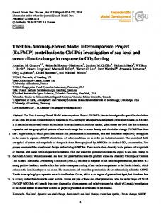
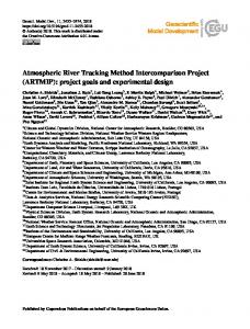
LSH tends to produce more soil moisture in the deeper layers especially when there is relatively little topography (less lateral flow) and when there is partial freezing. In the standard scheme under conditions of partial freezing deep in the soil the unfrozen soil moisture above is lowered. This is because gravitational drainage tends to lead to a small vertical gradient in unfrozen soil moisture. Hence the unfrozen soil moisture contents in the shallower layers are all effectively limited by the extent of soil moisture freezing in the deep layer. A sub-grid distribution of soil moisture and water table can be inferred from the sub-grid scale distribution in topography and mean soil moisture. This allows the calculation of partial inundation within each grid box, enhancing surface runoff. The estimate of inundation extent can also be used to diagnose a wetland fraction for calculating interactive wetland methane emissions (Gedney et al., 2004), for use by the chemistry scheme (Sect. 2.6). The wetland methane scheme requires a soil carbon content. This can be taken from the interactively derived values (Sect. 2.7). However, if anthropogenic land use changes are imposed (such as in the standard CMIP5 protocol), carbon can be added to or from the most labile soil carbon pool (see Sect. 2.7). This induces unrealistic changes in wetland methane emissions and hence in that case a soil carbon climatology needs to be used to drive the emissions. Feedbacks associated with changes in soil carbon, such as due to CO2 fertilisation (van Groenigen et al., 2011) are then not captured. As in HadCM3, the accumulation of frozen water on the permanent ice sheets is never returned to the freshwater cycle; that is, there is no representation of icebergs calving off ice shelves. To counterbalance these sinks in the global annual mean freshwater budget a freshwater flux field is applied to the ocean, with a pattern the same as that calibrated for HadCM3 but interpolated to the HadGEM2 ocean grid. Because there is no dynamic ice sheet modelling in HadGEM2 this calving flux does not vary with climate. Therefore if precipitation over ice sheets changes with time this will add or subtract from the snow depth and decrease or increase sea level. The freshwater fluxes are shown in Fig. 1. The scale used here is Sverdrup (Sv) which corresponds to 106 m3 s−1 or a change in sea level of ∼10 m per century. With the changes made to the conservation here and in Sects. 2.2 and 2.4, the fluxes are close to being in equilibrium. The exception to this is the atmosphere. The apparent imbalance in the atmosphere has been traced to a subtle difference between the diagnosed precipitation and the water removed from the atmosphere. 2.4

River model

The river scheme is based on TRIP (Oki and Sud, 1998) as in HadGEM1. It includes river transport dynamics, driven by fluxes of surface and subsurface runoff. TRIP operates on a 1◦ ×1◦ grid which is higher resolution than either www.geosci-model-dev.net/4/1051/2011/

W. J. Collins et al.: Development and evaluation of an Earth-System model – HadGEM2

1055

Fig. 1. Freshwater fluxes in HadGEM2 in Sv (106 m3 s−1 ) averaged over 10 yr of the model control run (pre-industrial conditions). Values inside the boxes are the differences between the flow in and out of each box.

the atmosphere or the land surface model, necessitating additional coupling to transfer the runoff fluxes and integrated river flows. The integrated river flows are deposited at predefined coastal outflow points on the atmosphere grid and then passed to the ocean model as a surface freshwater flux term. Errors in the formulation of this coupling led to a lack of water conservation in the HadGEM1 model. An additional loss of water was caused where rivers terminated in inland basins rather than at the coasts. In HadGEM2 this water is now added to the soil moisture at the location of the inland basin until this grid point becomes saturated. For saturated basins, water conservation is forced to be maintained by scaling the total coastal outflow. 2.5

Aerosols

Eight aerosol species are now available in HadGEM2. They are ammonium sulphate, ammonium nitrate, fossil-fuel black carbon, fossil-fuel organic carbon, mineral dust, biomassburning, sea salt and biogenic aerosols. The latter two are not transported but are diagnosed or provided as a climatology. Aerosols scatter and absorb solar and terrestrial radiation (direct effect), and provide the cloud droplet number (indirect effects). The aerosols are coupled with other components of the model, such as the vegetation scheme and the ocean model. The nitrate, fossil-fuel organic carbon and biogenic aerosols are new to HadGEM2. The biogenic aerosol climatology was found to reduce the continental warm bias www.geosci-model-dev.net/4/1051/2011/

thus improving the vegetation distribution (see Sect. 3.2 and Martin et al., 2010). Changes to the aerosol scheme since HadGEM1 are described in detail in Bellouin et al. (2011). The nitrate aerosols were added after the main model development and are not included in the CMIP5 integrations (Jones et al., 2011). Nitrate aerosols can only be included if the interactive tropospheric chemistry is used. All other species can be included without tropospheric chemistry. Important couplings that have been introduced into HadGEM2 are the provision of the oxidants that convert SO2 and DMS to sulphate and the provision of HNO3 as a precursor for nitrate aerosols. These sulphur oxidants (OH, H2 O2 , HO2 and O3 ) can be provided as climatological fields (the oxidation by O3 is new to HadGEM2), or taken from the interactive tropospheric chemistry scheme. The interactive coupling is important to simulate the changes in oxidation rates with climate change, and with the change in reactive gas emissions. It also ensures that the oxidant concentrations are consistent with the model meteorological fields. Modelled sulphate concentrations obtained with interactively simulated oxidants have been found to compare with observations at least as favourably as those obtained with prescribed oxidants. The nitric acid from the interactive chemistry generates ammonium nitrate aerosol with any remaining ammonium ions after reaction with sulphate. The sulphate and nitrate schemes deplete H2 O2 and HNO3 from the gas-phase chemistry. The introduction of these couplings permits investigations of climate-chemistry-aerosol feedbacks.

Geosci. Model Dev., 4, 1051–1075, 2011

W. J. Collins et al.: Development and evaluation of an Earth-System model – HadGEM2

2.6

Tropospheric chemistry

The atmospheric chemistry component of HadGEM2 is a configuration of the UKCA model (UK Chemistry and Aerosols; O’Connor et al., 2011) which includes tropospheric NOx -HOx -CH4 -CO chemistry along with some representation of non-methane hydrocarbons similar to the TOMCAT scheme (Zeng and Pyle, 2003). The 26 chemical tracers are included in the same manner as other model tracers. The chemical emissions from all anthropogenic sources, and most natural sources (including non-wetland methane), are provided as external forcing data (Jones et al., 2011). Interactive lightning emissions of NOx are included according to Price and Rind (1993). Photolysis rates are calculated offline in the Cambridge 2-D model (Law and Pyle, 1993). Dry deposition is an adaptation of the Wesely (1989) scheme as implemented in the STOCHEM model (Sanderson et al., 2006). A complete suite of tracer and chemical diagnostics has also been included. As the chemical scheme does not take account of halogen chemistry relevant to the stratoGeosci. Model Dev., 4, 1051–1075, 2011

Zonal mean methane (ppbv) 10

30

20 100

Pressure (hPa)

The facility to run the aerosol scheme with prescribed oxidants is still available for model configurations where aerosols, but not gas phase chemistry are required, such as the physics only HadGEM2-AO (HadGEM2 Development team, 2011). Mineral dust is a new species added to HadGEM2 and is important for its biogeochemical feedbacks. The dust model in HadGEM2 is based on Woodward (2001), but with significant improvements to the emission scheme (Woodward, 2011). Calculation of dust emission is based on the widelyused formulation of Marticorena and Bergametti (1995) for a horizontal flux size range of 0.03 to 1000 µm radius. Threshold friction velocity is obtained from Bagnold (1941) and the soil moisture dependence is based on Fecan et al. (1999). The vertical flux is calculated in 6 bins up to 30 µm radius. Dust affects both shortwave and longwave radiative fluxes, using radiative properties from Balkanski et al. (2007). It is removed from the atmosphere by both dry and wet deposition processes, providing a source of iron to phytoplankton and thus potentially affecting the carbon cycle. Dust is only emitted from the bare soil fraction of a gridbox, which in the Earth system configuration is calculated by the TRIFFID interactive vegetation scheme. This provides the coupling between vegetation and dust which is an important component of the biogeochemical feedback mechanisms which this model is designed to simulate. Inevitably, model simulated bare soil fraction is less realistic than the climatology and this has an undesirable impact on dust production, exacerbated by the increase in wind speed and drying of soil associated with loss of vegetation. In order to limit unrealistic source areas and so minimise this effect, whilst maintaining a sensitivity to climate-induced vegetation change, a preferential source term (Ginoux, 2001) has been introduced to limit dust emissions to areas of topographic depression.

Height (km)

1056

10

0 90N

0

45N

400

0 Latitude

800

1200

45S

1600

1750

90S

1850

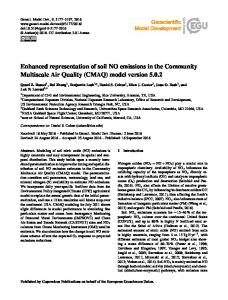
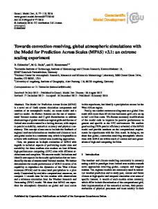
Fig. 2. Annually average zonal mean methane concentrations generated by the HadGEM2 chemistry driven with 2005 emissions of methane and ozone precursors from Jones et al. (2011).

sphere, stratospheric ozone concentrations are prescribed according to climatology from the CMIP5 database from 3 levels (3–5 km) above the tropopause. Methane loss in the stratosphere is parameterised with a 60 day decay time in the top three layers (above 28 km). The motivation for implementing a tropospheric chemistry, but not a stratospheric one, was based largely on the focus on biogeochemical couplings. These involve the oxidation of SO2 and DMS to form sulphate aerosol, the emissions of methane from wetlands and the radiative impacts of tropospheric ozone and methane. Stratospheric chemistry would not be useful unless the model top were raised and the vertical resolution in the stratospheric increased, both of which would slow the model. Interactive chemistry is computationally very expensive, due both to the advection of the many tracers and the integration of the chemical equations. For this reason only a simple tropospheric chemistry scheme could be afforded for centennial-scale climate integrations. The UKCA interactive chemistry in HadGEM2 takes methane emissions from wetlands generated by the largescale hydrology scheme (Sect. 2.3). The overall scaling was chosen to give emissions of approximately 130 Tg methane per year under pre-industrial conditions. The interactive gas-phase chemistry provides oxidants (HO2 , H2 O2 , and O3 ) and nitric acid (HNO3 ) to the aerosol scheme, which in turn depletes H2 O2 and HNO3 from the gas-phase. The three dimensional concentrations of ozone and methane are used by the radiation scheme. Methane had previously been implemented in the radiation scheme as a single value over the whole globe, and at all altitudes. Figure 2 shows that in HadGEM2, methane concentrations decrease rapidly above the tropopause. There is little transport into or out of the topmost model layer, so the concentrations there are essentially zero (Corbin and Law, 2011). In the 38 level configuration of the model, methane oxidation above the tropopause does not affect the stratospheric water vapour. www.geosci-model-dev.net/4/1051/2011/

W. J. Collins et al.: Development and evaluation of an Earth-System model – HadGEM2 2.7

Terrestrial carbon cycle

The terrestrial carbon cycle component of HadGEM2 is made up of the TRIFFID dynamic vegetation model (Cox, 2001; Clark et al., 2011) and an implementation of the RothC soil carbon model (Coleman and Jenkinson, 1999). The TRIFFID vegetation scheme had been used in a configuration from a previous generation of Hadley Centre models (HadCM3LC). It simulates phenology, growth and competition of 5 plant functional types (broad-leaved and needleleaved trees, C3 and C4 grasses and shrubs). An agricultural mask is applied to prevent tree and shrub growth in agricultural regions. This mask can vary in time in transient simulations allowing HadGEM2 to represent both biophysical and biogeochemical impacts of land use change. When the mask is applied to areas previously occupied by trees and shrubs, these areas are converted to bare soil and the carbon previously stored in the vegetation is moved to the most labile soil carbon pool. While there is no explicit crop plant functional type, these new bare soil areas can be taken over by the C3 and C4 grasses. There is no irrigation or harvesting applied to the grasses. A primary reason for including a dynamic vegetation model in HadGEM2 is to simulate the global distribution of fluxes and stores of carbon. Organic carbon is stored in the soil when dead litter falls from vegetation, either as dropped leaves or branches or when whole plants die. It is returned to the atmosphere as heterotrophic respiration when soil organic matter is decomposed by microbes. In HadGEM2 we have implemented the 4-pool RothC soil carbon model (Coleman and Jenkinson, 1999) which simulates differentiated turnover times of four different pools of soil carbon ranging from easily decomposable plant matter to relatively resistant humus. Multi-pool soil carbon dynamics have been shown to affect the transient response of soil carbon to climate change (Jones et al., 2005). Although each RothC pool currently has the same sensitivity to soil temperatures and moisture there is the ability to allow the model to enable different sensitivities for each pool as suggested by Davidson and Janssens (2006). Note that this model is not designed to simulate the large carbon accumulations in organic peat soils, or the stocks and dynamics of organic matter in permafrost. Global carbon stores are determined by the fluxes of carbon into and out of the vegetation/soil system. The fluxes “in” are due to vegetation productivity (supplied to TRIFFID from the surface exchange scheme), and the fluxes “out” due to vegetation and soil respiration. Productivity is frequently expressed as gross primary production (GPP) which is the total carbon uptake by photosynthesis, and net primary production (NPP) which is the difference between GPP and plant respiration (carbon released by the plant’s metabolism), parameterised as the sum of the growth and maintenance terms. The carbon cycle is closed by the release of soil respiration – decomposition of dead organic matter. In the absence of fires or time-varying land use, the net flux (net ecosystem exwww.geosci-model-dev.net/4/1051/2011/

1057

change, NEE, or net ecosystem productivity, NEP) is therefore given by GPP-total respiration. A comprehensive calibration of the terrestrial ecosystem parameters has been undertaken to improve the carbon fluxes compared to HadCM3LC, some of which have been described in Sect. 2.2. The Q10 temperature response function of soil heterotrophs was kept from HadCM3LC, rather than using the generic function in RothC (which leads to too low soil respiration in winter). In addition the soil respiration is now driven by soil temperatures from the second soil layer instead of the first layer as in HadCM3LC, as most of the decomposable soil carbon would be on average at this depth. This leads to a smaller seasonal cycle in soil temperatures, and thus reduced seasonality in soil respiration without affecting long-timescale sensitivity to temperature. The response of soil respiration to moisture is represented by the total soil moisture (frozen plus unfrozen), compensating for a cold bias in high latitude winter soil temperatures (due to insufficient insulation of soil under snow (Wiltshire, 2006)). Seasonality in leaf phenology of temperate ecosystems, and thus seasonal plant productivity, is improved by delaying the onset of the growing season relative to HadCM3LC using a 5 ◦ C growing degree base for the deciduous vegetation phenology, as used in Sitch et al. (2003). This contributes to an improved simulation of photosynthesis. The above changes are described in more detail in Cadule et al. (2010). While the transport of atmospheric tracers in HadGEM2 is designed to be conservative, the conservation is not perfect and in centennial scale simulations this non-conservation becomes significant. This has been addressed by employing an explicit “mass fixer” which calculates a global scaling of CO2 to ensure that the change in the global atmospheric mean mass mixing ratio of CO2 in the atmosphere matches the total flux of CO2 into or out of the atmosphere each timestep (Corbin and Law, 2010). 2.8

Ocean carbon cycle

The ocean biogeochemistry component in HadGEM2 provides the ocean component of the carbon cycle and the provision of di-methyl sulphide (DMS) emissions from phytoplankton. It consists of an ecosystem model and related submodels for seawater carbon chemistry and the air-sea transport of CO2 , the cycling of iron supplied by atmospheric dust, and the production and sea-to-air transfer of DMS. The ecosystem model used is the Diat-HadOCC model, a development of the previous HadOCC model (Palmer and Totterdell, 2001) that splits the phytoplankton compartment into “diatoms” and “other phytoplankton”. Diatoms require silicate to form their shells, are very sensitive to ironlimitation, do not produce significant amounts of DMS, but do form a disproportionately large part of the sinking flux of fixed carbon to the deep ocean. Modelling diatoms as a separate compartment is therefore tractable (because of their Geosci. Model Dev., 4, 1051–1075, 2011

1058

W. J. Collins et al.: Development and evaluation of an Earth-System model – HadGEM2

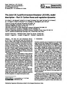
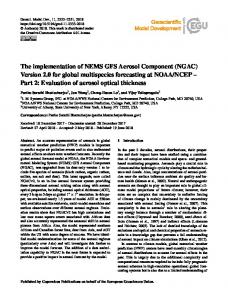
Fig. 3. Earth system couplings feedbacks.

requirement for silicate) and allows an improved representation of the biological pump and of DMS production. Iron, carbon, dissolved inorganic nitrogen and silicate are transported as three dimensional tracers in the ocean. Iron is now recognised as an important micro-nutrient for phytoplankton, which can limit growth in some areas of the ocean (including the Southern Ocean and parts of the North and Equatorial Pacific). In many ocean areas iron found in the surface waters has mainly been supplied by atmospheric dust deposition (the Southern Ocean is an exception), and although utilisation by phytoplankton can be a temporary sink this iron is quickly recycled and the long-term removal process is transfer to the sediments via adsorption onto mineral particles. Modelling iron cycling in the ocean allows us to examine possible climate feedbacks whereby increased dust production improves iron availability in the ocean, strengthening the biological pump and increasing the uptake of CO2 by the ocean. DMS, which is a significant source of sulphate aerosol over the oceans, is produced within Diat-HadOCC using the parameterisation of Simo and Dachs (2002) as described in Halloran et al. (2010). This scheme relates the DMS production to surface water chlorophyll concentrations and the depth of the corresponding mixed layer.

Geosci. Model Dev., 4, 1051–1075, 2011

3 3.1

Developing the coupled model Couplings in HadGEM2

One of the prime motivations for incorporating Earth system processes, which cannot be achieved with offline modelling, is to include Earth system couplings (Fig. 3). Combinations of these couplings form biogeochemical feedback loops. The couplings take place every dynamical timestep (30 min in this configuration) within the land-atmosphere system, except for those involving radiation which take place every 3 h. Coupling between the ocean and the atmosphere is on a daily timescale. The vegetation distributions are updated every 10 days. All components are driven by the physical climate. The gas-phase chemistry is coupled to the aerosol scheme through the provision of concentrations of OH, H2 O2 and O3 for the oxidation of SO2 and DMS, and is coupled to the radiation scheme through the provision of three dimensional concentrations of O3 and CH4 . The aerosols are coupled to the cloud microphysics and the radiation scheme. The dust deposition is coupled to the ocean biogeochemistry and supplies iron nutrient. There is no impact of the aerosols on the chemistry, e.g. through heterogeneous reactions or effect on the photolysis rates, except that the aqueous-phase SO2 oxidation depletes H2 O2 in the chemistry and the nitrate aerosol formation (when used) depletes the gas phase HNO3 .

www.geosci-model-dev.net/4/1051/2011/

W. J. Collins et al.: Development and evaluation of an Earth-System model – HadGEM2 The land ecosystems determine the exchange of CO2 between the land and the atmosphere. They are coupled to the physical climate through the vegetation distribution and leaf area index which affects the surface albedo, the stomatal conductance which determines the evapotranspiration flux, and the roughness length which affects the surface wind and momentum transport. The vegetation cover controls the dust emissions, and the wetland model supplies methane emissions to the atmospheric chemistry. Surface removal (dry deposition) of gas-phase chemical species and aqueous-phase aerosols also depends on the vegetation cover and stomatal conductance. Other emissions of trace gases and aerosols from the terrestrial biosphere such as from vegetation, soils and fires are not considered. As well as determining the ocean-atmosphere exchange of CO2 , the ocean biogeochemistry scheme provides a flux of DMS into the atmosphere, thus providing a source of sulphate aerosol precursor. Many feedback loops can be constructed from Fig. 3, and hence can be examined in HadGEM2 configurations. Numerous studies (e.g. Friedlingstein et al., 2006; Sitch et al., 2008) have looked at the loop from the climate impacts on ecosystems to the CO2 concentrations and back to climate. The Charlson, Lovelock, Andreae, Warren (CLAW) hypothesis (Charlson et al., 1987) described a loop from climate to ocean biogeochemistry, sulphate aerosols, cloud microphysics and to climate. In HadGEM2-ES this can be extended by starting the CLAW loop by following the coupling from climate to terrestrial vegetation, dust emissions, iron deposition and the fertilisation of the ocean biogeochemistry. Future experiments will quantify the individual feedback pathways through breaking coupling loops in specific places by replacing exchanged quantities with prescribed fields. 3.2

Development and spin up

When combining multiply connected model components there are numerous possibilities for biases in one place to disrupt the evaluation in another. In extreme cases this could lead to runaway feedbacks where components drive each other further and further from a realistic representation of the observed state. In the HadGEM2 development process, each Earth system component was initially developed separately from the others by being coupled only to the physical atmosphere or ocean, with the other components represented by climatological data fields. Only when all the individual components proved to be stable and realistic were these data fields replaced by interactive couplings. An example of this was the interaction between the surface climate and the dynamic vegetation. The TRIFFID scheme was initially tested in the HadGEM1 physical climate model. The model had a very low soil moisture (compared the previous generation of Met Office Hadley Centre models such as HadCM3LC) in the summertime in the centres of the northern continents (central and northern Asia., central and northwww.geosci-model-dev.net/4/1051/2011/

1059

ern North America). This dryness reduced the growth of vegetation; however with less vegetation the soils dried out further. This process eventually led to the decline of all vegetation in these regions and extreme summer temperatures and dryness. The increase in the summertime continental soil moisture was one of the improvements made to the physical model in the development from HadGEM1 to HadGEM2 (Martin et al., 2010). In parallel the TRIFFID model was developed in a configuration driven by observed meteorology where improvements were made to give a more realistic tolerance to arid conditions. Before being finally combined, TRIFFID was driven offline by meteorology from the HadGEM2 physical model. This ensured the final coupled configuration was stable. The components were spun up to 1860 climate conditions, which we refer to as “pre-industrial”, by imposing emissions or concentrations of gases and aerosols as specified by the CMIP5 project (see Jones et al., 2011). The species for which concentrations were imposed are N2 O, halocarbons and stratospheric ozone. We assumed the climate system to be approximately in equilibrium at this time. The Earth system components with long timescales (decade or more) are the ocean physical and nutrient variables, the vegetation distribution, the soil carbon content and the methane concentrations. The deep ocean circulation operates on timescales of millennia or tens of millennia. In practice, we chose to spin up to a state where drifts over the length of an expected model experiment (around 300 yr) were small. Drifts can be accounted for in experimental setups by running a control integration parallel to the experiment. The TRIFFID vegetation scheme has a fast spin up mode in which it can use an implicit timestep to take 100 yr jumps every 3 model years. After the physical and vegetation improvements described above, a near-stable distribution in the coupled system is achieved after 12 model years (equivalent to 400 vegetation years) for 1860 conditions. The fast spin up of vegetation cover is not fully successful at spinning up the soil carbon stores, because sub-annual fluctuations in the litter inputs are of comparable magnitude to changes in the small, rapid-turnover decomposable plant material pool which subsequently affects the long-lived humified organic matter pool. Hence, an offline spin-up of the soil carbon model was carried out to spin up the least labile soil carbon store of humified organic matter (e-folding time of around 50 yr). Using monthly mean diagnostics of litter inputs and rate modifying factors the soil carbon model was run offline for 2000 yr until all the pools had reached steady state. A final equilibration of vegetation cover and soil carbon storage was then achieved by running the model with TRIFFID in its normal, real-time mode for a further 10–20 yr with fixed atmospheric CO2 (286 ppm). This distribution is evaluated in Sect. 4.4 and found to be suitable for carbon cycle modelling, but leads to an over prediction of dust compared to simulations using the IGBP vegetation climatology (Sect. 4.2.2). Geosci. Model Dev., 4, 1051–1075, 2011

1060

W. J. Collins et al.: Development and evaluation of an Earth-System model – HadGEM2 Atm surface CO2

300

Land Carbon 1600

295

1590

290 GtC

ppm

1580 285

1570 280 1560

275 270

1550 0

50

100

150 year

200

250

300

0

50

Ocean Primary Production 40

150 year

200

250

300

250

300

0.6

38

0.4 0.2

36

GtC/yr

GtC/yr

100

air-to-sea CO2 flux

34

0.0 -0.2 -0.4

32

-0.6

30 0

50

100

150 year

200

250

300

0

50

100

150 year

200

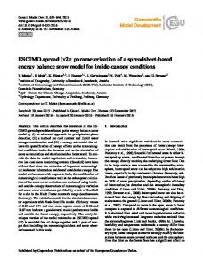
Fig. 4. Atmospheric CO2 , land carbon store, ocean primary productivity and the air to sea CO2 flux from 280 yr of the HadGEM2 control integration under 1860 conditions.

Fig. 5. Methane concentrations from the spin up of the chemistry components under 1860 conditions. JJA obs wetland (Prigent) 90N

JJA obs wetland (Prigent)

To ensure stability when all Earth system components were combined, this over predicted dust was used in the spin up of the ocean biogeochemistry. The physical ocean was initialised from a control run from the previous (HadGEM1) climate model (Johns et al., 2006) with biogeochemical fields from HadCM3LC (C and N) or Garcia et al. (2010) for Si. Fe was initialised to a constant value. The ocean was spun up first for 400 yr in an oceanonly configuration with forcings (meteorology, atmospheric CO2 , dust input) provided as external driving fields. After this time the upper ocean nutrients and vertically integrated primary productivity had stabilised. The ocean was coupled back to the atmosphere and the composition fields (DMS, dust). With the components of the carbon cycle now equilibrated, the constraint on the atmospheric CO2 concentrations could be removed and the model allowed to reach its own equilibrium. Figure 4 shows the carbon cycle variables from 280 yr of the control integration following the spin up. This uses continuous 1860 forcing conditions. Trends are very small, particularly in the atmospheric CO2 concentrations, showing that the system has successfully spun up. There is a slight increase in the land carbon of about 5 Gt(C) after 280 yr. This would correspond roughly to a decrease in the atmospheric concentration of 0.01 ppm per yr which is negligible compared to any anthropogenically-forced experiments. The air to sea CO2 flux is close to zero, confirming that the terrestrial and oceanic carbon fluxes have equilibrated. Of the gas-phase and aerosol chemical constituents, only methane has a long enough lifetime to require spinning up. For the core CMIP5 control run (Jones et al., 2011), methane surface concentrations were specified rather than interactively calculated so little spin up was needed. However for the model to be suitable for further investigations Geosci. Model Dev., 4, 1051–1075, 2011

90N 45N 45N 0 0 45S 45S 90S 180

90W

0

90E

90S 180 0.025

0.05

0.1

0 0.2

0.3

0.4

0.025

0.05

0.1

0.2

0.3

0.4

90W

90E

JJA Modelled wetland 90N

JJA Modelled wetland 90N 45N 45N

0 0

45S 45S 90S 180 90S 180

90W

0

90W

90E

0

90E

0.025

0.05

0.1

0.2

0.3

0.4

0.025

0.05

0.1

0.2

0.3

0.4

Fig. 6. June-July-August average inundation fraction: (a) satellite observations (Prigent et al., 2001, b) HadGEM2 model.

of methane feedbacks we need to create a spun up interactive methane distribution. From the model lifetime (8.9 yr) and an observed 1860 concentration, the expected methane emission rate was calculated. The anthropogenic component www.geosci-model-dev.net/4/1051/2011/

W. J. Collins et al.: Development and evaluation of an Earth-System model – HadGEM2 Coastal River Discharge - Observations (Sv)

Coastal River Discharge - HadGEM2-ES (Sv)

90N

90N

45N

45N

0

0

45S

45S

90S 180

90W

5e-4

0.002

0

90E

0.01

0.05

180

1061

90S 180

0.2

90W

5e-4

0.002

0

90E

0.01

0.05

180

0.2

Fig. 7. Mean annual (1948–2004) discharge (Sv) from 4◦ latitude by 5◦ longitude coastal box estimated from available gauge records and reconstructed river flow (Dai et al., 2009) and simulated discharge from HadGEM2.

was 59 Tg yr−1 , oceans and termites totalled 45 Tg yr−1 , so the wetland component was adjusted to give the required total (237 Tg yr−1 ). This was run for 15 yr to verify that the methane concentrations were close to the observed 805 ppb (see Fig. 5).

4

Evaluation of components

The long-timescale Earth system components (terrestrial and ocean carbon cycles) were developed under 1860 conditions as described in Sect. 3, which limited the comparisons that could be carried out at that stage. The model has now been run through the historical period (Jones et al., 2011) thus allowing comparison with present day observations. The aerosols and chemistry equilibrate on sufficiently short timescales that they could be developed and evaluated in atmosphere-only configurations of the model forced with AMIP sea surface temperatures and sea ice (Gates et al., 1999). Martin et al. (2010) evaluates the impacts of the developments to the physical model. Of particular note are the improvements to the northern summertime surface temperatures and the net primary productivity (their Figs. 13 and 17). Further physical evaluation is available in The HadGEM2 Development Team (2011). 4.1

Land surface hydrology and the river model

The land surface hydrology model provides runoff for the river flow model and also predicts inundation area for use in the wetland emission scheme (Sect. 4.3). Figure 6 compares the modelled northern hemisphere summer inundation fraction against that derived from an Earth observations product (Prigent et al., 2001). The model distribution is much smoother than the satellite product which has very localised areas with high inundation fractions. Some inundation areas such as central Canada seem to be missing from the model. The model significantly over-estimates inundation www.geosci-model-dev.net/4/1051/2011/

extent over the Amazon basin. This is probably due to poor data on the underlying rock topography in this region as used in the driving topographic dataset. Rivers provide significant freshwater input to the oceans thereby forcing the oceans regionally through changes to density. The inclusion of the TRIP river flow model allows the inclusion of this regional ocean forcing, which is an important component of both Earth system and atmosphereocean models. The total HadGEM2-ES simulated discharge to the oceans is 1.07 Sv, within the observational range of 1.035 to 1.27 Sv (Dai and Trenberth, 2002) but tending to the low side. Figure 7 compares the simulated regional discharge from HadGEM2-ES and an observational dataset of ocean discharge from Dai et al. (2009). HadGEM2-ES simulates the point of river discharge in a slightly different location to the observations due to the smoothed land-sea mask of the ocean model. However, the major rivers such as the Amazon, Ganges/Brahmaputra and Mississippi are all well simulated. 4.2

Aerosols

The improved aerosols in HadGEM2 have been extensively evaluated in Bellouin et al. (2007, 2011) and The HadGEM2 Development Team (2011). Here we focus specifically on the biogeochemical couplings between aerosols and the oceanic and terrestrial ecosystems through emissions of DMS and mineral dust. DMS is emitted by ocean phytoplankton and is oxidised in the atmosphere to form sulphate aerosol and methane sulphonic acid (MSA). In the HadGEM2 aerosol scheme, MSA is assumed not to form aerosols. In the open oceans, DMS is the predominant precursor of sulphate aerosol. Figure 8 shows comparisons between observed and simulated atmospheric DMS concentrations at 3 sites in the Southern Hemisphere for which the prevailing air masses come from the open ocean. The simulations are with both interactive ocean biology (HadGEM2-ES) and prescribed sea water DMS concentrations (HadGEM2-AO). The interactive scheme seems Geosci. Model Dev., 4, 1051–1075, 2011

1062

W. J. Collins et al.: Development and evaluation of an Earth-System model – HadGEM2 Dust load (mg m-2)

DMS concentrations at Amsterdam Island 90N

1.0 Observations HadGEM2-AO HadGEM2-ES

0.8 μg[S]/m3

45N 0.6

0

0.4 0.2

45S 0.0 J

F

M

A

M

J J Month

A

S

O

N

D

90S 180

DMS concentrations at Dumont d’Urville

90W

0

90E

180

1.0 Observations HadGEM2-AO HadGEM2-ES

μg[S]/m3

0.8

0

0.6

20

100

500

2000

1e+4

Fig. 9. Modelled decadal mean dust load in HadGEM2-ES for 1991–2000.

0.4 0.2 0.0 J

F

M

A

M

J J Month

A

S

O

N

D

O

N

D

DMS concentrations at Cape Grim 1.0 Observations HadGEM2-AO HadGEM2-ES

μg[S]/m3

0.8 0.6 0.4 0.2 0.0 J

F

M

A

M

J J Month

A

S

Fig. 8. Comparison of DMS concentrations in the southern mid and high latitudes with the HadGEM2 simulations; with (HadGEM2ES) and without (HadGEM2-AO) interactive ocean biology. Observations are from Ayers et al. (1991), Jordain et al. (2001) and Nguyen et al. (1992). For Amsterdam Island the shaded area spans the 5–95 % range of the observations, for Dumont d’Urville it spans the ±2 standard deviation range. For Cape Grim only the mean concentrations are available.

to over predict the austral winter atmospheric concentrations compared to using the prescribed sea water concentrations. This is in spite of the good comparison between the simulated and observed ocean concentrations (as seen later in Sect. 4.5 and Fig. 21). This suggests that there may be regional differences in the emissions. At the Antarctic station of Dumont d’Urville, the interactive scheme does better at simulating the austral summer concentrations. As seen in Fig. 21, the Kettle et al. (1999) climatology used to prescribe DMS overestimates these concentrations. Dust production is highly sensitive to various atmospheric and surface variables, and the introduction and coupling together of new biogeochemical components – particularly interactive vegetation – in the Earth system model will inevitably lead to changes in these variables, not all of which Geosci. Model Dev., 4, 1051–1075, 2011

Fig. 10. Comparison of modelled (HadGEM2-ES) and observed near surface dust concentrations and total aerosol optical depths (AODs) at 440 nm. Observed optical depths are from AERONET stations in dust-dominated regions and concentrations from stations of the University of Miami network (with thanks to J. M. Prospero and D. L. Savoie). Symbols indicate: crosses – AODs, stars – Atlantic concentrations, squares – N Pacific concentrations, triangles – S Pacific concentrations, diamonds – Southern Ocean concentrations.

enhance the simulation of dust emissions. Thus dust fields are not expected to be as close to reality as in a more constrained model. Despite this, the global dust distribution in HadGEM2-ES (Fig. 9) is broadly realistic. Figure 10 shows a comparison of modelled and observed near-surface dust concentrations and aerosol optical depths in dust-dominated locations. Good agreement is seen for dust from Saharan www.geosci-model-dev.net/4/1051/2011/

W. J. Collins et al.: Development and evaluation of an Earth-System model – HadGEM2

1063

Difference in dust load (mg m-2)

90N

Difference in dust load (mg m-2)

Kagoshima ( 31.4 N,130.4 E)

Irene ( 25.2 S, 28.2 E)

90N 45N

0 45S

200

400

HadGEM2 CMIP5 Observations

600

Pressure / hPa

Pressure / hPa

200

45N 0

800

45S 90S 180

0

90E

90S 180 -1000

-200

-50

-10

10

50

200

180 1000

-1000

-200

-50

-10

10

50

200

1000

90W

0

90E

1000 10

100 1000 10000 Ozone / ppbv Sapporo ( 43.0 N,141.2 E)

180

400

HadGEM2 CMIP5 Observations

600 800

Difference in bare soil fraction 90N 45N 45N 0

90E

180

90W -0.6

0

90E 0.6

180 1

-0.4

-0.2

0.2

0.4

0.8

400

HadGEM2 CMIP5 Observations

600

-0.8

-0.6

-0.4

-0.2

0.2

0.4

0.6

0.8

400

HadGEM2 CMIP5 Observations

600

1000

1000 100 1000 Ozone / ppbv

10000

10

100 1000 Ozone / ppbv

10000

1

Fig. 11. Differences in dust load (above) and bare soil fraction (below) between HadGEM2-ES and an atmosphere-only simulation (HadGEM2-A) forced by AMIP SSTs, using fixed vegetation from IGBP. Values are decadal means 1991–2000.

sources, though concentrations in the Pacific are somewhat too high. This is due to excess dust from areas where an unrealistically high bare-soil fraction, combined with the consequent drying of the surface and increase in wind speed, have caused anomalous emissions, particularly in Australia, India and the Sahel (Fig. 11). Despite these limitations, the global dust load is sufficiently well represented for the purpose of investigating the biogeochemical feedback processes involving dust. Interactive emission schemes are unlikely to perform as well as using prescribed emissions. However they allow us to include feedbacks between the biological components and the atmospheric composition, and make predictions of future levels of emissions. Evaluation of Chemistry Component of HadGEM2

Figure 12 shows comparisons of July vertical ozone profiles from the HadGEM2 interactive chemistry run compared with the ozone climatology supplied for the CMIP5 project (Lamarque et al., 2010) and climatological observations at a subset of sites from Logan (1999). Data are compared for www.geosci-model-dev.net/4/1051/2011/

100 1000 10000 Ozone / ppbv Edmonton ( 53.5 N,113.3 W)

800

10

-1

10

200

800

-0.8

HadGEM2 CMIP5 Observations

600

10000

Pressure / hPa

0

Pressure / hPa

90W

4.3

100 1000 Ozone / ppbv Alert ( 82.3 N, 62.2 W)

200

90S 180 -1

400

1000 10

45S 90S 180

100 1000 10000 Ozone / ppbv Tateno ( 36.0 N,140.1 E)

800

1000

0 45S

10

200 Pressure / hPa

90N

Pressure / hPa

200

Difference in bare soil fraction

HadGEM2 CMIP5 Observations

600 800

1000

90W

400

Fig. 12. Comparison of modelled July vertical ozone profiles with climatological observations (black) from Logan 1999), interactive chemistry (red) and the CMIP5 ozone concentrations (blue).

1990–1994 in each case. The HadGEM2 data are taken from a transient run. Note that we used the same anthropogenic emissions of ozone precursors as were used by Lamarque et al. to generate the CMIP5 climatology. The comparison indicates that the vertical ozone profiles from HadGEM2 and the CMIP5 datasets compare well with observations. From 3 km above the tropopause, the interactive ozone values are relaxed to the CMIP5 climatology. The HadGEM2 ozone concentrations near the tropical tropopause are higher than in the CMIP5 climatology due to a lower ozone tropopause in HadGEM2 (diagnosed from the 150 ppb contour). This leads to slightly higher tropical tropopause temperatures when using the interactive ozone. The wetland methane emissions are shown in Fig. 13. As well as the major tropical wetlands, there are significant boreal emissions during the northern summer. The global total is 137 Gt (CH4 ) yr−1 . 80 % of the emissions are in the tropics which is a higher fraction than from other bottom-up studies (e.g. Walter et al., 2001), but within the range of the various inversion top-down studies (O’Connor et al., 2010). Even though there is considerable uncertainty in the geographical magnitudes of emissions it is likely that the large model Geosci. Model Dev., 4, 1051–1075, 2011

1064

W. J. Collins et al.: Development and evaluation of an Earth-System model – HadGEM2 Wetland emissions (g(C)m-2yr-1) Model DJF

Wetland emissions (g(C)m-2yr-1) Bousquet DJF

90N

90N

45N

45N

0

0

45S

45S

90S 180

0.1

90W

0.2

0.5

0

1

90E

2

5

10

180

90S 180

20

0.1

Wetland emissions (g(C)m-2yr-1) Model JJA 90N

45N

45N

0

0

45S

45S

0.1

90W

0.2

0.5

0

1

90E

2

5

10

0.2

0.5

0

1

2

90E

5

10

180

20

Wetland emissions (g(C)m-2yr-1) Bousquet JJA

90N

90S 180

90W

180

90S 180

20

0.1

90W

0.2

0.5

0

1

2

90E

5

10

180

20

Fig. 13. Distribution of emissions of methane from wetlands provided to the HadGEM2 chemistry scheme by the large-scale hydrology, compared to those from an inversion study (Bousquet et al., 2006).

2000

CH4 / ppbv

1900 1800 1700 1600

Measurements HadGEM2-ES

1500 90

60

30

0 Latitude

-30

-60

-90

Fig. 14. Comparison of modelled methane concentrations for the 1990s compared with observations from a selection of sites from NOAA ESRL (Dlugokencky et al., 2011).

emissions over Amazonia are due to the over-estimate of the modelled inundation extent (see Sect. 4.1). The seasonal patterns of the modelled wetland fluxes are compared qualitatively against those of an inversion study (Bousquet et al., 2006) in Fig. 13. It should be noted that the spatial pattern here derives mainly from the data used (Matthews and Fung, 1987) as the prior for the inversion. Geosci. Model Dev., 4, 1051–1075, 2011

The locations of the seasonal maxima for most of the Northern mid and high latitudes are consistent between the model and the inversion. The differences between modelled and observed inundation areas previously shown in Fig. 6 can also be seen as differences in the wetland methane emissions. The movement of the zone of maximum methane emissions over Central Africa follow similar seasonal patterns. Over S.E. Asia there is considerable disagreement in the magnitude of natural wetland fluxes. This is likely to be due to difficulties in separating man-made and natural inundation (Chen and Prinn, 2006). The latitudinal variation in the surface methane concentration is shown in Fig. 14, and is compared against surface measurements from NOAA ESRL (Dlugokencky et al., 2011). The agreement at the individual sites is reasonable, although the latitudinal gradient is slightly weaker in the model. The methane lifetime for present day (2005) conditions is 8.8 yr; in good agreement with previous studies (Stevenson et al., 2006). 4.4

Terrestrial carbon cycle

In the model development stage we evaluated and calibrated the simulation of the terrestrial carbon cycle by HadGEM2 in a pre-industrial control phase, with atmospheric CO2 held fixed at 290 ppmv. It would have been much too computationally expensive to perform repeated 140 yr historical www.geosci-model-dev.net/4/1051/2011/

W. J. Collins et al.: Development and evaluation of an Earth-System model – HadGEM2 Tree cover: IGBP

0.1

0.2

0.4

0.6

0.2

0.4

0.6

0.8

1

0.1

0.2

0.8

0.2

0.4

0.6

0.4

0.6

0.8

1

0.1

0.2

0.4

1

0.1

0.2

0.4

0.6

0.8

1

0.1

0.2

0.4

Grass/shrub cover: HadCM3LC

0.8

1

0.1

0.2

0.4

0.6

0.8

0.6

0.8

1

Bare soil: HadGEM2-ES

Grass/shrub cover: HadGEM2-ES

Tree cover: HadCM3LC

0.1

Bare soil: IGBP

Grass/shrub cover: IGBP

Tree cover: HadGEM2-ES

0.1

1065

0.6

0.8

1

Bare soil: HadCM3LC

1

0.1

0.2

0.4

0.6

0.8

1

Fig. 15. IGBP Climatology and HadGEM2-ES simulation of tree cover (defined as the total of both broadleaf and needleleaf tree), grass, shrub and bare soil.

Soil Carbon: IGBP

Soil Carbon: HadGEM2-ES

90N

90N

45N

45N

0

0

45S

45S

90S 180

90W

0

5

0

10

90S 180

90E

15

20

25

90W

0

5

0

10

90E

15

20

25

25

Soil Carbon: HadCM3LC

20

90N kgC m-2

45N 0

IGBP HadGEM2-ES HadCM3LC

15 10

45S 5

90S 180

90W

0

90E 0 90N

0

5

10

15

20

25

60N

30N 0 Latitude

30S

60S

Fig. 16. Climatological (Zinke et al., 1986) and simulated (HadGEM2-ES top right, HadCM3LC bottom left) soil carbon distributions. Bottom right shows a comparison of the zonal means of these distributions.

www.geosci-model-dev.net/4/1051/2011/

Geosci. Model Dev., 4, 1051–1075, 2011

1066

W. J. Collins et al.: Development and evaluation of an Earth-System model – HadGEM2 system over the period 1860-present. Hence we also show here a comparison of the model state with the final parameter setup from a transient historical climate simulation with climate forcings representative of the 20th century implemented as described by Jones et al. (2011). Developing the terrestrial carbon cycle model within the pre-industrial control phase may lead to some discrepancy between the eventual HadGEM2 present-day simulation and observed datasets. We demonstrate here that the model performance is sufficiently good to make HadGEM2 fit for purpose.

1200

Vegetetaion Carbon / GtC

1000

800

600

400

200

4.4.1 0 0

500

1000 1500 Soil Carbon / GtC

2000

2500

Fig. 17. Present day global total soil and vegetation carbon (GtC) from the 11 C4 MIP models (black crosses) and HadGEM2-ES (red star) compared with estimated global totals of: biomass (Olson et al., 1985, present 2 central estimates of global vegetation carbon (dashed horizontal lines) and high and low confidence limits – dotted); soil carbon (Prentice et al., 2001, state a global estimate of 1350 GtC not including inert soil carbon – dashed vertical line). In the absence of estimated uncertainty range for soil carbon we choose ±25 % as a reasonable tolerance (dotted lines).

4•10-8

Potsdam ±3s.d. MODIS Pre-industrial HadGEM2-ES Present day HadGEM2-ES

kgC m-2 s-1

3•10-8

2•10-8

1•10-8

0 90N

60N

30N

0

30S

60S

Latitude

Fig. 18. Zonal mean distribution of NPP from HadGEM2-ES (preindustrial simulation in blue, present day simulation in red) compared with datasets of global NPP from the Potsdam model database (black) with ±3 standard deviations (shaded) and MODIS (Heinsch et al., 2003; black dashed).

simulations for the different parameter combinations in order to evaluate the model against present day observations. The main aim is to assess how well the model performs and whether it is fit for purpose as an Earth System model, but we also make use of a comparison against HadCM3LC simulations as a benchmark and, where available, some data from the range of C4 MIP coupled climate-carbon cycle models (Friedlingstein et al., 2006). Such a comparison is inherently imperfect due to the significant changes in the Earth Geosci. Model Dev., 4, 1051–1075, 2011

Vegetation cover

It is still rare for dynamic vegetation models to be coupled within climate GCMs. In C4 MIP only 2 out of the 11 models were GCMs with dynamic vegetation, and both of those had some form of climate correction term such as ocean heat flux adjustment to enable the vegetation simulation to be sufficiently realistic. HadGEM2 dynamically simulates vegetation without a need for any flux-correction to its climate state. The vegetation simulation of HadGEM2 compares favourably with observed land cover maps and is generally a little better than that simulated by HadCM3LC. We compare present day conditions from transient simulations of HadCM3LC (as performed for C4 MIP; Friedlingstein et al., 2006) and HadGEM2-ES (as performed for CMIP5; Jones et al., 2011) with the observed IGBP climatology (Loveland et al., 2000). Agricultural disturbance is representative of present day. Figure 15 shows the observed and simulated total tree cover, grass and shrub cover and bare soil. For broadleaf trees (not shown separately) HadGEM2-ES is generally a little better than HadCM3LC, especially in temperate latitudes where it correctly simulates some coverage in the mixed forest areas to the southern edge of the boreal forest zone. In the tropics both GCMs have a tendency to simulate too much tropical forest, although this excess is lower in HadGEM2ES: the latter also has an improved coverage in the north east of Brazil where HadCM3LC has a gap in the forest. For needleleaf trees HadGEM2-ES simulation is similar to that of HadCM3LC. Neither model correctly simulates the area of cold-deciduous larch forest in east Siberia whose phenology is not well represented in TRIFFID. Overall HadGEM2ES does a good job at simulating the global distribution of trees. Grass and shrub are generally simulated better than in HadCM3LC which had much too great coverage in the high latitudes. This comes though at the expense of simulating too little shrub and too much grass. Inclusion of an agricultural mask to prevent trees growing in areas of present day agriculture results in the model being able to represent well the main agricultural regions of North America, Europe and Asia. The HadGEM2-ES simulation is now better in temperate zones and central Africa but there is too little coverage in Australia. www.geosci-model-dev.net/4/1051/2011/

W. J. Collins et al.: Development and evaluation of an Earth-System model – HadGEM2 NEP

GPP 400 gC m-2 month-1

gC m-2 month-1

200 100 0 -100 -200

300 200 100 0

0

2

4

6 Month

8

10

12

0

2

4

NPP

8

10

12

8

10

12

8

10

12

400 gC m-2 month-1

gC m-2 month-1

6 Month

Plant Resp.

400 300 200 100 0

300 200 100 0

0

2

4

6 Month

8

10

12

0

2

4

Soil Resp.

6 Month

Total Resp. 400 gC m-2 month-1

400 gC m-2 month-1

1067

300 200 100 0

300

HadGEM2-ES

200

HadCM3LC

100

Obs.

0 0

2

4

6 Month

8

10

12

0

2

4

6 Month

Fig. 19. Observed and simulated carbon fluxes at Harvard Forest site, USA. HadGEM2-ES (red), HadCM3LC (green). Observations are the mean of 8 yr from AMERIFLUX, .(http://public.ornl.gov/ameriflux/)

Bare soil is diagnosed from the absence of simulated vegetation. HadGEM2-ES captures the main features of the world’s deserts, and is better than the previous simulation of HadCM3LC except in Australia where it now simulates too great an extent of bare soil. The main tropical deserts are captured as before, but now HadGEM2-ES also simulates better representation of bare soil areas in mid-latitudes and the south western USA. As before, the simulated Sahara/Sahel boundary is slightly too far south. Along with Australia, there is also too much bare soil in western India in common with HadCM3LC. The presence of too much bare soil in Australia causes problems for the dust emissions scheme. 4.4.2

Simulation of terrestrial carbon stores

Correctly simulating the correct magnitude of global stores of carbon is essential in order to be able to simulate the effect of climate on carbon storage. If the model simulates much too much or too little terrestrial carbon then the impact of climate will be over or under estimated. Jones and Falloon (2009) show the strong relationship between changes in soil organic carbon and the overall magnitude of climate-carbon cycle feedback. www.geosci-model-dev.net/4/1051/2011/

Figure 16 shows the observed (Zinke et al., 1986) and simulated distribution of soil carbon. Both HadGEM2-ES and HadCM3LC models do a reasonable job at representing the main features with HadGEM2-ES improved in the extra-tropics but now over-representing slightly the observed soil carbon in the tropics (especially in Brazil and southern Africa). Insufficient vegetation in Siberia and Australia leads inevitably to too little soil carbon in those regions, which previously had too much. Global total soil carbon is estimated as about 1500 GtC but with considerable uncertainty (Prentice et al., 2001). HadGEM2-ES simulates 1107 GtC globally for the period 1979–2003, while HadCM3LC simulates 1200 GtC. Considering that about 150 GtC of the observed estimate will be more inert carbon (not represented in our models) and that the models are not yet designed to simulate the large carbon accumulations in organic peat soils, it may be expected that the simulations underestimate the global total. The range of simulated soil carbon from the 11 C4 MIP models is 1040–2210 GtC, so HadGEM2-ES lies comfortably within this range (Fig. 17) although towards the lower end. Both models also do a reasonable job at representing the main features of global vegetation carbon storage (not Geosci. Model Dev., 4, 1051–1075, 2011

1068

W. J. Collins et al.: Development and evaluation of an Earth-System model – HadGEM2

Control run: geographical location of histogram bins

log(Control run surface chl.)

90N 0.125 45N

-0.875 -1.875

0

-2.875 45S

-3.875

90E

180

90W

-4.875 0.0

0

SeaWiFs: geographical location of histogram bins

0.2 0.4 0.6 0.8 normalised frequency

1.0

log(SeaWiFS surface chl.)

90N 0.125 45N

-0.875 -1.875

0

-2.875 45S

-3.875

90E

180

-4.5

90W

-4.875 0.0

0

-3.75 -3 -2.25 -1.5 -0.75 0 bin centre log(chlorophyll) mg/m2

0.2 0.4 0.6 0.8 normalised frequency

1.0

0.75

Fig. 21. Observed (Keeling et al., 2008; black) and simulated seasonal cycles of atmospheric CO2 (in ppm) comparing HadGEM2ES (red) and HadCM3LC (blue) for Mauna Loa (left) and Barrow (right).

W. J. Collins et al.: Development and evaluation of an Earth-System model – HadGEM2

Fig. 20. Comparison of model-generated chlorophyll surface concentrations (top) with observations from SeaWiFs (bottom). The left hand side shows maps whereas the right hand side shows histograms of the statistics on each grid square. The quantity plotted is the log of the concentration in each case.

Geosci. Model Dev., 4, 1–25, 2011ww.geosci-model-dev.net

Fig. 20. Comparison of model-generated chlorophyll surface concentrations (top) with observations from SeaWiFs (bottom). The left hand side shows maps whereas the right hand side shows histograms of the statistics on each grid square. The quantity plotted is the log of the concentration in each case.

1.0

0.2 0.4 0.6 0.8 normalised frequency

1.0

0.2 0.4 0.6 0.8 normalised frequency

log(SeaWiFS surface chl.)

-4.875 0.0

90E

45S

0

45N

90N

-3.75 -3 -2.25 -1.5 -0.75 0 bin centre log(chlorophyll) mg/m2 -4.5

180

90W

0

0.75

-3.875

-2.875

0.125

-1.875

-0.875

-4.875 0.0

SeaWiFs: geographical location of histogram bins

-3.875

-2.875

0 90W 180 90E

log(Control run surface chl.)

0.125

-0.875

-1.875

0

45S

12 10 8

0

100

200

300

400

0

2

4

6 Month

Soil Resp.

Control run: geographical location of histogram bins

gC m-2 month-1

Geosci. Model Dev., 4, 1051–1075, 2011

as Siberia now have too low biomass. Globally, vegetation carbon is estimated to be between 450 and 550 GtC but this has very large uncertainty with upper and lower ranges estimated at around 270 GtC and 900 GtC (Olson et al., 1985). HadGEM2-ES now simulates 478 GtC compared with 530 GtC in HadCM3LC for the period 1979–2003 – both well within a realistic range. For comparison the equivalent range from the C4 MIP models was 350–970 GtC (Fig. 17). The main areas of disagreement between observed 45N

Obs.

2

0

100

200

300

0

2 0 12 10

0

100

200

300

400

-200

0

-100

0

2

4

NPP

6 Month

8

10 8

6 Month 2

4

NEP

100

0

gC m-2 month-1

200

400

0

100

200

300

400

100

200

gC m-2 month-1

24

gC m-2 month-1

300

0

gC m-2 month-1

12

gC m-2 month-1

400

0

2

shown) although they have a tendency to underestimate biomass in regions of low amounts. Unlike soil carbon, simulation of vegetation carbon is much more sensitive to errors in simulated vegetation cover. HadGEM2-ES has an improved simulation of the biomass per unit area of the Amazon forest which was previously a little low in HadCM3LC, but it now overestimates the total tropical biomass due to having too great an extent of forest. Similarly areas where we have already noted deficient simulated vegetation such

90N

Fig. 19. Observed and simulated carbon fluxes at Harvard Forest site, USA. HadGEM2-ES (red), HadCM3LC (green). Observations are the mean of 8 yr from AMERIFLUX, .(http://public.ornl.gov/ ameriflux/)

12

6 Month 4

HadGEM2-ES

HadCM3LC

8

10

12 10 8

6 Month

Total Resp.

4

6 Month 4

GPP

Plant Resp.

8

10

12

Fig. 21. Observed (Keeling et al., 2008; black) and simulated seasonal cycles of atmospheric CO2 (in ppm) comparing HadGEM2-ES (red) and HadCM3LC (blue) for Mauna Loa (left) and Barrow (right).

www.geosci-model-dev.net/4/1051/2011/

W. J. Collins et al.: Development and evaluation of an Earth-System model – HadGEM2 HadGEM2-ES - HadGEM2-AO JJA 1.5m temperature (K) 90N 45N

0

45S 90S 180 -4

90W -3

-2

0 -1

-0.5

90E 0.5

1

2

180 3

4

Fig. 22. Comparison of 1.5 m temperatures between the earth system (-ES) and physics-only (-AO) configurations of HadGEM2. Data are 20 yr averages for the boreal summer (June, July and August).

and simulated biomass are due to errors in simulated vegetation cover, but there also exist errors in biomass for each vegetation type such as slight over prediction of biomass in tropical trees and under prediction of biomass in conifers and grasses 4.4.3

Simulation of vegetation productivity

Component carbon fluxes are hard to measure directly, but some datasets do exist. Point observations of component fluxes exist such as from flux tower data from the EUROFLUX (Valentini, 2002) and AMERIFLUX (http:// public.ornl.gov/ameriflux/) projects. Global products of NPP and GPP exist but are model based and not directly observed. The Potsdam dataset (Cramer et al., 1999) is a global, gridded product derived from the mean NPP simulations of 17 terrestrial ecosystem models driven by observed climate. NPP products are also available from remote sensing such as that derived from the MODIS satellite (Heinsch et al., 2003). However, to process satellite-observed radiances into estimates of NPP requires complex algorithms (Zhao et al., 2005) and is subject to errors in the same way as estimates from land-surface models. While process modelling and remote sensing give comparable estimates of global NPP values, neither approach has been able to reduce uncertainty to within around 10 GtC yr−1 with mean estimates for present day global NPP of about 55–60 GtC yr−1 (Ito, 2011). Figure 18 shows the zonal distribution of global NPP from several model configurations compared with the model mean NPP from the Potsdam intercomparison (Cramer et al., 1999). The Potsdam dataset also provides the standard deviation of model results about the mean, and a comparison of the dataset with site level observations shows that ±3 standard deviation is an appropriate estimate of uncertainty. MODIS NPP is also plotted (annual mean for 2000–2006; dashed www.geosci-model-dev.net/4/1051/2011/

1069

line). This is systematically lower than Potsdam estimates and coincides closely in the zonal mean with Potsdam-3σ . We do not know the reason for this difference but it highlights the large uncertainty involved in measuring vegetation productivity (Zhao et al., 2005). The figure shows separate lines for HadGEM2-ES from pre-industrial and present day. As described earlier the preindustrial simulation was the only simulation available for evaluation during the development stage. During calibration HadGEM2-ES was developed to simulate a good match to the multimodel climatology. The pre-industrial line in Fig. 18 is slightly below the Potsdam model. Due to increased atmospheric CO2 , global NPP has increased substantially during the 20th century and the present day simulation of HadGEM2-ES can be seen to be higher than the preindustrial one, and generally within the Potsdam estimates. Table 2 shows that HadGEM2-ES simulates an increase of 22 % during this period. This is at the top end, but within the range of increase simulated by the 11 C4 MIP models of 0.4–23 %. A comparison of HadGEM2-ES with a simulation of HadGEM2-A (an atmosphere-only simulation with prescribed sea-surface temperature and vegetation cover) is shown in The HadGEM2 Development Team (2011). The HadGEM2-A simulated NPP is generally lower than HadGEM2-ES and most of this difference is due to climate differences rather than differences in vegetation cover. Table 2 shows the global total NPP values from various datasets and model simulations. HadGEM2-ES simulates reasonable present day productivity and is generally of comparable skill to HadCM3LC for the distribution of annual mean NPP. HadGEM2-ES performs much better for the amplitude of the seasonal cycle of NEP and other component carbon fluxes at monitoring stations, whereas HadCM3LC had some large errors in this respect (Cadule et al., 2010). Figure 19 illustrates the flux components at one of these sites, Harvard Forest. At Harvard Forest HadGEM2-ES now better simulates both component fluxes and the net seasonal cycle, capturing the summer draw down due to the later onset of growth and lower summer respiration. Both models are better at reproducing the seasonality of fluxes in forested ecosystems than at sites representing water limited ecosystems, e.g. grasslands and Mediterranean ecosystems. HadGEM2-ES has an improved phase in the seasonal cycle of GPP compared with HadCM3LC which consistently simulated too early onset of spring uptake, and has an improved peak-season amplitude. Improvements to the seasonal cycle of NEP lead to a much improved simulation of the seasonal cycle of atmospheric CO2 at monitoring stations such as Mauna Loa (see Sect. 4.6). Across the flux sites considered, HadGEM2-ES has a lower normalised RMS error than HadCM3LC for GPP, respiration and NEP. We conclude that for both the simulation of the seasonal cycle of component carbon fluxes and the global distribution of simulated NPP, the combined improvements Geosci. Model Dev., 4, 1051–1075, 2011

1070

W. J. Collins et al.: Development and evaluation of an Earth-System model – HadGEM2

Table 2. Global total net primary productivity, NPP (GtC yr−1 ) from observationally derived estimates (Potsdam dataset (Cramer et al., 1999), and MODIS), a model and observations meta-analysis (Ito, 2011) and global models. For the Potsdam dataset we quote the standard deviation, and for C4 MIP we quote the range across the 11 models. The “-ES” and “-A” refer to the full Earth system, and to physical atmosphere-only configurations of HadGEM2. Potsdam

MODIS

Meta-analysis

pre-industrial present-day

HadGEM2 -A

58.0 60.9 ± 6.9

48.6

56.0 ± 14.3

% increase

described in Sect. 2.7 lead HadGEM2-ES to perform better than previously seen in HadCM3LC. Although this does not necessarily imply an improved simulation of changes in the terrestrial carbon cycle it gives confidence that the underlying processes have been improved during the model development. Systematic attempts to benchmark land surface models are being developed (e.g. Randerson et al., 2009; Cadule et al., 2010; Blyth et al., 2011) – the challenge is to be able to understand how such model evaluations lead to constraints on the projections from these models. 4.5

HadGEM2 -ES

Ocean biogeochemistry

The ocean biogeochemistry is evaluated when coupled with the dynamic vegetation model and the interactive dust scheme. This means that iron input into the ocean from wind-borne dust is driven by the bare soil areas generated by the vegetation scheme. Figure 20 shows a comparison of the annual mean chlorophyll surface concentration with that observed from SeaWiFs. The modelled values are calculated by scaling the plankton abundances assuming a carbon to chlorophyll ratio of 40. There is generally a good correlation except for the centres of the ocean gyres where the model has very low nutrient levels. The vertical distribution of productivity in the model peaks at the surface, whereas in reality the peak is slightly deeper. Hence in the observations, the satellite does not see the peak levels so the modelled concentrations are considerably higher although the patterns are reproduced.. The total productivity is 36 Gt(C)yr−1 , with diatoms responsible for 55 % of the total primary production. Estimates of global annual productivity from remotely-sensed data range from below 40 to greater than 60 Gt(C)yr−1 (Carr et al., 2006). So the Diat-HadOCC model has production that is around or below the lower bound. Note that the observed values include high levels of production near the coasts which we are not trying to simulate with the open ocean biology. The original HadOCC model running in the same conditions has a global total of 53 Gt(C)yr−1 . The difference between standard HadOCC and Diat-HadOCC production is Geosci. Model Dev., 4, 1051–1075, 2011

70.5

54.6

21.6 %

HadCM3LC

C4 MIP

62.4

52.9–75.7

68.9

54.1–82.2

10.4 %

0.4–23.3 %

mainly due to the additional limitation on growth due to iron. The North Pacific and Southern Ocean show iron limitation during their respective summers, the Equatorial Pacific is affected by iron limitation throughout the year and the North Atlantic is never iron-limited (because of high dust inputs from the Sahara). In contrast, the first three areas mentioned are never limited by the macro-nutrients (nitrogen and silicate) in the model, but growth in the temperate North Atlantic shows seasonal macro-nutrient limitation. All these patterns of limitation are similar to those observed; giving confidence that the vegetation-dust-plankton coupled system can generate realistic productivity distributions. The global percentage of primary production that is due to diatoms, 55 %, is slightly above the estimate of 40 % given by Tr´eguer et al. (1995). The pattern of total primary production is reasonable, with high seasonal production in the sub-polar regions and low production in the large sub-tropical gyres. The spatial distribution of model DMS production in most basins correlates well with that inferred from the standard DMS climatology (Kettle et al., 1999), however due to the small size of the dataset from which this climatology was produced, the climatology itself represents only a first order estimate of global ocean DMS values. This performance of the DMS scheme is analysed in detail in Halloran et al. (2010) which finds that the modelled DMS values are closer to observations, than those presented in the Kettle et al. climatology. 4.6

Carbon Cycle simulations

Atmospheric transport integrates the large scale responses of the terrestrial and ocean carbon cycles. Hence atmospheric CO2 observations at measurement sites are a valuable source of evaluation data for HadGEM2 at the global scale. In this section we assess the behaviour of the carbon cycle in HadGEM2-ES, with the atmospheric CO2 concentrations determined by the carbon fluxes from the terrestrial and ocean ecosystem components. The seasonal cycle in the model is particularly dependent on the balance between the NPP and the soil respiration. The improvements to the terrestrial carbon fluxes described in Sect. 2.7 give very good agreement between the simulated and observed atmospheric CO2 www.geosci-model-dev.net/4/1051/2011/

W. J. Collins et al.: Development and evaluation of an Earth-System model – HadGEM2 concentrations. As shown in Fig. 21, the seasonal cycle is much better in HadGEM2-ES compared to HadCM3LC. We compare simulated and observed seasonal cycle of CO2 at two commonly used CO2 flask measurement sites, Mauna Loa in Hawaii, and Pt. Barrow in Alaska. At both sites, HadCM3LC had significant errors in phase and magnitude, as noted by Cadule et al. (2010). HadGEM2-ES shows better agreement with the observed seasonal cycle. At Mauna Loa the magnitude agrees better with observations as does the timing of the seasonal minimum in September/October, although the observed seasonal maximum in May is still simulated 1 month too early in HadGEM2-ES. At Pt Barrow, HadGEM2-ES captures improved timing of both cross-over dates and the summer peak drawdown, although the magnitude is now slightly too high.

5

Impact of Earth system components on the physical climate

The physical climate of HadGEM2 without the Earth system components (HadGEM2-AO) has been evaluated in Martin et al. (2010) and The HadGEM2 Development Team (2011). The interactive Earth system components generally replace datasets that are specified in HadGEM2-AO as climatologies compiled from observed data. This allows us to understand how feedbacks in the Earth system may affect our predictions of future climate change. Introducing interactive components rather than using climatologies inevitably degrades the overall simulation of the present day climate since no interactive scheme is perfect. However by allowing these components to vary with climate an Earth system model may provide more realistic future predictions. The two Earth system components having the largest effect on the simulation of the present physical climate are the vegetation scheme and the chemistry scheme. In this section we quantify their impact on the ability to simulate present climate. The vegetation cover simulated by TRIFFID in HadGEM2 is generally good, but has some deficiencies as described in Sect. 4.4, in particular a lack of vegetation in India and Australia, as well as north and east Siberia, where the model simulates too much bare soil. The model also tends to simulate an overly strong southward extent of tropical forest into savannah areas, probably due to lack of anthropogenic or fire disturbance. These features have implications for other Earth system components, especially the emission of dust from the land surface as discussed in Sect. 4.2. Simulations with and without interactive vegetation show little overall difference in the surface climate. Surface temperatures are shown in Fig. 22. There are indications of slightly reduced summer land surface temperatures in Siberia where more bare soil leads to higher albedo. However, these do not seem to have a significant effect on the large scale circulation or other surface climate variables (The HadGEM2 Development Team, 2011), and we conclude that the model www.geosci-model-dev.net/4/1051/2011/

1071

simulation of physical climate is not significantly degraded by the inclusion of a dynamic vegetation scheme. The interactive chemistry scheme determines the concentrations of tropospheric ozone and methane that are used by the model radiation scheme. The increased tropospheric ozone at the tropical tropopause in the interactively simulated ozone compared to the CMIP5 climatology leads to increased temperatures in this region. The impact of the much lower stratospheric methane concentrations with the interactive chemistry has negligible effect on the stratospheric temperatures. This is presumably because ozone and CO2 dominate the radiative effects at this altitude. There was no discernable impact on global-scale climate patterns from using the interactive chemistry in the radiation scheme. As well as affecting the atmospheric CO2 levels, the ocean biology affects the climate through the DMS emissions, which increase sulphate aerosol formation, which in turn affects cloud properties. The non-Earth system configuration of HadGEM2 (The HadGEM2 Development Team, 2011) uses a DMS surface water climatology from Kettle et al. (1999). As shown in Halloran et al. (2010), the interactive scheme generates lower DMS emissions in the southern ocean than the Kettle et al. (1999) climatology and is more in line with recent observations. Comparisons between simulations with interactive DMS and with the Kettle climatology show some indication of lower amounts and less bright low cloud in the Southern Ocean with the Earth system configuration. However it was not possible to detect any difference in temperature or precipitation. Overall the addition of the Earth system components does not significantly affect the representation of the climate state. Further comparison between the HadGEM2 family members can be found in The HadGEM2 Development Team (2011). 6

Conclusions

In the HadGEM2 model family, the addition of Earth system components to the Hadley Centre climate model provides the ability to understand the contributions of biogeochemical feedbacks to the future evolution of the climate system. In selecting the components to include we have concentrated on those where coupling processes are expected to have the largest effect on the climate. These components are the carbon cycle and short-lived forcing agents (gas and aerosol phase). Inevitably model development involves pragmatic decisions and some potentially important processes have been excluded (such as the nitrogen cycle). The extra complexity in Earth system models leads to increased uncertainty in their predictions. However, given that we have an expectation that biogeochemical feedbacks are occurring in reality, this increased uncertainty is a more realistic assessment of our knowledge of the future evolution of the climate. A major achievement of the HadGEM2 model development process has been the construction of a stable model Geosci. Model Dev., 4, 1051–1075, 2011

1072

W. J. Collins et al.: Development and evaluation of an Earth-System model – HadGEM2

that represents a realistic state (corresponding to 1860 conditions) of the climate, vegetation and ocean biology with no need for artificial corrections terms. Results from a transient model integration following the CMIP5 protocol suggest that the representation of present day conditions is also satisfactory. Given the numerous interactions between components and the scope for large feedback loops, this outcome was not obvious at the start of the project. Although the overall performance of the model is good, there are some areas where deficiencies are amplified by the coupling processes. An example we have shown of this is the under prediction of vegetation in some arid areas which leads to a large over prediction of dust emissions. The difference between using interactive Earth system components compared to using climatological representations compiled from observations has impacts on physical climate variables. These impacts in HadGEM2 appear to be confined to specific variables (such as cloud albedo in the case of DMS emissions) and do not appear to make a significant difference to the overall representation of climate. The HadGEM2 development has produced an Earth system model that is proving a useful science tool to predict future climate and understand the climate feedbacks within the Earth system. It is being run to generate results for the CMIP5 intercomparison with all the components included and coupled except the nitrate aerosol scheme (Jones et al., 2011). The creation of the HadGEM2 model family means that it is not necessary to run with all components for all purposes. For instance, to assess climate forcing from aerosols a configuration without the ocean components is run, using climatologies prepared from the fully coupled integrations to supply the necessary fields (Bellouin et al., 2011). Acknowledgements. The development of the HadGEM2 family represents the work of a large number of people, to whom the authors are indebted. This work was supported by the Joint DECC/Defra Met Office Hadley Centre Climate Programme (GA01101). CDJ and SL were additionally supported under the COMBINE EU FP7 project. Edited by: O. Marti

References Ayers, G., Ivey, J., and Gillett, R.: Coherence between seasonal cycles of dimethylsulfide, methanesulfonate, and sulfate in marine air, Nature, 349, 404–406, 1991. Bagnold, R. A.: The Physics of Blown Sand and Desert Dunes, Methuen, New York, 1941. Balkanski, Y., Schulz, M., Claquin, T., and Guibert, S.: Reevaluation of Mineral aerosol radiative forcings suggests a better agreement with satellite and AERONET data, Atmos. Chem. Phys., 7, 81–95, doi:10.5194/acp-7-81-2007, 2007. Bellouin, N., Boucher, O., Haywood, J., Johnson, C., Jones, A., Rae, J., and Woodward, S.: Improved representation of aerosols for HadGEM2, Hadley Centre Technical Note No. 73, 2007.

Geosci. Model Dev., 4, 1051–1075, 2011

Bellouin, N., Rae, J., Johnson, C., Haywood, J., Jones, A., and Boucher, O.: Aerosol forcing in the Hadley Centre CMIP5 simulations by HadGEM2-ES and the role of ammonium nitrate, J. Geophys. Res., 116, D20206, doi:10.1029/2011JD016074, 2011. Best, M. J., Pryor, M., Clark, D. B., Rooney, G. G., Essery, R .L. H., M´enard, C. B., Edwards, J. M., Hendry, M. A., Porson, A., Gedney, N., Mercado, L. M., Sitch, S., Blyth, E., Boucher, O., Cox, P. M., Grimmond, C. S. B., and Harding, R. J.: The Joint UK Land Environment Simulator (JULES), model description – Part 1: Energy and water fluxes, Geosci. Model Dev., 4, 677– 699, doi:10.5194/gmd-4-677-2011, 2011. Beven, K. J. and Kirkby, M.J.: A physically based, variable contributing area model of basin hydrology, Hydrol. Sci. Bull., 24, 43–69, 1979. Blyth, E., Clark, D. B., Ellis, R., Huntingford, C., Los, S., Pryor, M., Best, M., and Sitch, S.: A comprehensive set of benchmark tests for a land surface model of simultaneous fluxes of water and carbon at both the global and seasonal scale, Geosci. Model Dev., 4, 255–269, doi:10.5194/gmd-4-255-2011, 2011. Booth, B. B. B., and Jones, C. D.: Terrestrial response of QUMPC ensemble. Hadley Centre Technical Note, 89, 2011. Bousquet, P., Ciais, P., Miller, J. B., Dlugokencky, E.J., Hauglustaine, D.A., Prigent, C., Van der Werf, G.R., Peylin, P., Brunke, E.-G., Carouge, C., Langenfelds, R.L., Lathi`ere, J., Papa, F., Ramonet, M., Schmidt, M., Steele, L.P., Tyler, S.C., and White, J.: Contribution of anthropogenic and natural sources to atmospheric methane variability, Nature, 443, 439–443, 2006. Cadule, P., P. Friedlingstein, Bopp, L., Sitch, S., Jones, C. D., Ciais, P., Piao, S. L., and Peylin P.: Benchmarking coupled climate-carbon models against long-term atmospheric CO2 measurements, Glob. Biogeochem. Cy., 24, GB2016, doi:10.1029/2009GB003556, 2010. Carr, M.-E., Friedrichs, M. A. M, Schmeltz, M., Aita, M. N., Antoine, D., Arrigo, K. R., Asanuma, I., Aumont, O., Barber, R., Behrenfeld, M., Bidigare, R., Buitenhuis, E. T., Campbell, J., Ciotti, A., Dierssen, H., Dowell, M., Dunne, J., Esaias, W., Gentili, B., Gregg, W., Groon, S., Hoepffner, N., Ishizaka, J., Kameda, T., Le Quere, C., Lohrenz, S., Marra, J., Melin, F., Moore, K., Morel, A., Reddy, T. E., Ryan, J., Scardi, M., Smyth, T., Turpie, K., Tilstone, G., Waters, K., and Yamanaka, Y.: A comparison of global estimates of marine primary production from ocean color, Deep Sea Res. Pt. II: Topical Studies in Oceanography Volume 53, 5–7, 741–770, 2006. Charlson, R. J., Lovelock, J. E., Andreae, M. O., and Warren, S. G.: Oceanic phytoplankton, atmospheric sulphur, cloud albedo and climate, Nature, 326, 655–661, doi:10.1038/326655a0, 1987. Chen, Y.-H. and Prinn, R. G.: Estimation of atmospheric methane emissions between 1996 and 2001 using a three-dimensional global chemical transport model, J. Geophys. Res., 111, D10307, doi:10.1029/2005JD006058, 2006. Clark, D. B. and Gedney N.: Representing the effects of subgrid variability of soil moisture on runoff generation in a land surface model, J. Geophys. Res., 113, D10111, doi:10.1029/2007JD008940, 2008. Clark, D. B., Mercado, L. M., Sitch, S., Jones, C. D., Gedney, N., Best, M. J., Pryor, M., Rooney, G. G., Essery, R. L. H., Blyth, E., Boucher, O., Harding, R. J., Huntingford, C., and Cox, P. M.: The Joint UK Land Environment Simulator (JULES), model description – Part 2: Carbon fluxes and vegetation dynamics,

www.geosci-model-dev.net/4/1051/2011/

W. J. Collins et al.: Development and evaluation of an Earth-System model – HadGEM2 Geosci. Model Dev., 4, 701–722, doi:10.5194/gmd-4-701-2011, 2011. Coleman, K. and Jenkinson, D. S.: RothC-26.3, A model for the turnover of carbon in soil: Model description and User’s guide Lawes Agricultural Trust Harpenden, UK, 1999. Corbin, K. D. and Law, R. M.: Extending Atmospheric CO2 and Tracer Capabilities in ACCESS. CAWCR Technical Report No. 035, Centre for Australian Weather and Climate Research, Australia, http://www.cawcr.gov.au/publications/ technicalreports/CTR 035.pdf, 2010. Cox, P.M.: Description of the TRIFFID Dynamic Global Vegetation Model Hadley Centre, Met Office, Technical Note 24, 2001. Cox, P. M., Betts, R. A., Jones, C. D., Spall, S. A., and Totterdell, I. J.: Acceleration of global warming due to carbon-cycle feedbacks in a coupled climate model, Nature 408, 184–187 , doi:10.1038/35041539, 2000. Cramer, W., Kicklighter, D.W., Bondeau, A., Moore III, B., Churkina, G., Nemry, B., Ruimy, A., Schloss, A. L., and The Participants of the Potsdam NPP Model Intercomparison: Comparing global models of terrestrial net primary productivity (NPP): overview and key results, Glob. Change Biol., 5, S1, 1–15, 1999. Dai, A. and Trenberth, K. E.: Estimates of freshwater discharge from continents: Latitudinal and seasonal variations. J. Hydrometeorol., 3, 660–687, 2002. Dai, A., Qian, T., Trenberth, K. E., and Milliman, J. D.: Changes in continental freshwater discharge from 1948–2004, J. Climate, 22, 2773–2791, 2009. Davidson, E. and Janssens, I.: Temperature sensitivity of soil carbon decomposition and feedbacks to climate change, Nature, 440, 165–173, 2006. Dlugokencky, E. J., Lang, P. M., and Masarie, K. A.: Atmospheric Methane Dry Air Mole Fractions from the NOAA ESRL Carbon Cycle Cooperative Global Air Sampling Network, 1983–2010, Version: 2011-08-11, ftp://ftp.cmdl.noaa.gov/ccg/ ch4/flask/event/, 2011, Essery, R. L. H., Best, M.J., Betts, R. A., Cox, P. M., and Taylor, C. M.: Explicit representation of subgrid heterogeneity in a GCM land surface scheme, J. Hydrometeorol., 4, 530–543, 2003. Eyring, V., Butchart, N., Waugh, D. W., Akiyoshi, H., Austin, J., Bekki, S., Bodeker, G. E., Boville, B. A., Bruhl, C., Chipperfield, M. P., Codero, E., Dameris, M., Deushi, M., Fioletov, V. E., Frith, S. M., Garcia, R. R., Gettelman, A., Giorgetta, M. A., Grewe, V., Jourdain, L., Kinnison, D. E., Mancini, E., Manzini, E., Marchand, M., Marsh, D.R., Nagashima, T., Newman, P. A., Nielsen, J. E., Pawson, S., Pitari, G., Plummer, D. A., Rozanov, E., Schraner, M., Shepherd, T. G., Shibata, K., Stolarski, R. S., Struthers, H., Tian, W., and Yoshiki, M.: Assessment of temperature, trace species, and ozone in chemistry-climate model simulations of the recent past, J. Geophys. Res., 111, D22308, doi:10.1029/2006JD007327, 2006. Fecan, F., Marticorena, B., and Bergametti, G.: Parameterisation of the increase of the Aeolian erosion threshold wind friction velocity due to soil moisture for arid and semi-arid areas, Ann. Geophys., 17, 149–157, 1999, http://www.ann-geophys.net/17/149/1999/. Friedlingstein, P., Cox, P., Betts, R., Bopp, L., von Bloh, W., Brovkin, V., Cadule, P., Doney, S., Eby, M., Fung, I., Bala, G., John, J., Jones, C., Joos, F., Kato, T., Kawamiya, M., Knorr, W., Lindsay, K., Matthews, H.D., Raddatz, T., Payner, P., Reick,

www.geosci-model-dev.net/4/1051/2011/

1073

C., Roeckner, E., Schnitzler, K.G., Schnur, R., Strassmann, K., Weaver, A. J., Yoshikawa, C., and Zeng, N.: Climate-carbon cycle feedback analysis, results from the C4MIP model intercomparison. J. Climate, 19, 3337–3353 doi:10.1175/JCLI3800.1, 2006. Garcia, H. E., Locarnini, R. A., Boyer, T. P., Antonov, J. I., Zweng, M. M., Baranova, O. K., and Johnson, D. R.: World Ocean Atlas 2009, 4, in: Nutrients (phosphate, nitrate, silicate), edited by: S. Levitus, Ed. NOAA Atlas NESDIS 71, U.S. Government Printing Office, Washington, D.C., 398 pp., 2010. Gates, W. L., Boyle, J. S., Covey, C., Dease, C. G., Doutriaux, C. M., Drach, R. S., Fiorino, M., Gleckler, P. J., Hnilo, J. J., Marlais, S. M., Phillips, T. J., Potter, G. L., Santer, B. D., Sperber, K. R., Taylor, K. E., and Williams, D. N.: An overview of the results of the Atmospheric Model Intercomparison Project (AMIP I), B. Am. Meteor. Soc., 80, 29–55, 1999. Gedney, N. and Cox, P. M.: The sensitivity of global climate model simulations to the representation of soil moisture heterogeneity, J. Hydrometeorol., 4 1265–1275, 2003. Gedney, N., Cox, P. M., and Huntingford, C.: Climate feedback from wetland methane emissions, Geophys. Res. Lett., 31, L20503, doi:10.1029/2004GL020919, 2004. Ginoux, P., Chin, M., Tegen, I., Prospero, J. M., Holben, B., Dubovik, O., and Lin, S.-J.: Sources and distributions of dust aerosols simulated with the GOCART model, J. Geophys. Res., 106, D17, 20255–20273, 2001. Halloran, P. R., Bell, T. G., and Totterdell, I. J.: Can we trust empirical marine DMS parameterisations within projections of future climate?, Biogeosciences, 7, 1645–1656, doi:10.5194/bg-71645-2010, 2010. Heinsch, F. A., Reeves, M., Votava, P., Kang, S., Milesi, C., Zhao, M., Glassy, J., Jolly, W. M., Loehman, R., Bowker, C. F., Kimball, J. S., Nemani, R. R., and Running, S. W.: Users Guide GPP and NPP (MOD17A2/A3) Products NASA MODIS Land Algorithm. Version 2.0. University of Montana, Missoula, MT, 2003. Ito, A.: A historical meta-analysis of global terrestrial net primary productivity: are estimates converging? Glob. Change Biol., 17, 3161–3175, doi:10.1111/j.1365-2486.2011.02450.x, 2011. Jogireddy, V., Cox, P., Huntingford, C., Harding, H., and Mercado, L. M.: An improved description of canopy light interception for use in a GCM land-surface scheme: calibration and testing against carbon ?uxes at a coniferous forest, Hadley Centre Technical Note 63, Hadley Centre, Met Office, 2006. Johns, T. C., Durman, C. F., Banks, H. T., Roberts, M. J., McLaren, A. J., Ridley, J. K., Senior, C. A., Williams, K. D., Jones, A., Rickard, G. J., Cusack, S., Ingram, W. J., Crucifix, M., Sexton, D. M. H., Joshi, M. M., Dong, B.-W., Spencer, H., Hill, R. S. R., Gregory, J. M., Keen, A. B., Pardaens, A. K., Lowe, J. A., BodasSalcedo, A., Stark, S., and Searl, Y.: The new Hadley Centre climate model HadGEM1: Evaluation of coupled simulations, J. Climate, 19, 1327–1353, 2006. Jones, C. D., McConnell, C., Coleman, K. W., Cox, P., Falloon, P. D., Jenkinson, D., and Powlson, D.: Global climate change and soil carbon stocks; predictions from two contrasting models for the turnover of organic carbon in soil, Global Change Biol., 11, 154–166, doi:10.1111/j.1365-2486.2004.00885.x, 2005. Jones, C. D., Cox, P. M., and Huntingford, C.: Climate-carbon cycle feedbacks under stabilization: uncertainty and observational constraints, Tellus B, 8, 603–613, 2006.

Geosci. Model Dev., 4, 1051–1075, 2011

1074

W. J. Collins et al.: Development and evaluation of an Earth-System model – HadGEM2

Jones, C., Lowe, J., Liddicoat, S., and Betts, R.: Committed terrestrial ecosystem changes due to climate change, Nature Geosci., 2, 484–487 doi:10.1038/ngeo555, 2009. Jones, C. D., and Falloon, P.: Sources of uncertainty in global modelling of future soil organic carbon storage, in “Uncertainties in environmental modelling and consequences for policy making”, edited by: Baveye, P., Mysiak, J., and Laba, M., Springer, Germany, 2009. Jones, C. D., Hughes, J. K., Bellouin, N., Hardiman, S. C., Jones, G. S., Knight, J., Liddicoat, S., O’Connor, F. M., Andres, R. J., Bell, C., Boo, K.-O., Bozzo, A., Butchart, N., Cadule, P., Corbin, K. D., Doutriaux-Boucher, M., Friedlingstein, P., Gornall, J., Gray, L., Halloran, P. R., Hurtt, G., Ingram, W. J., Lamarque, J.-F., Law, R. M., Meinshausen, M., Osprey, S., Palin, E. J., Parsons Chini, L., Raddatz, T., Sanderson, M. G., Sellar, A. A., Schurer, A., Valdes, P., Wood, N., Woodward, S., Yoshioka, M., and Zerroukat, M.: The HadGEM2-ES implementation of CMIP5 centennial simulations, Geosci. Model Dev., 4, 543–570, doi:10.5194/gmd-4-543-2011, 2011. Jourdain, B. and Legrand, M.: Seasonal variations of atmospheric dimethylsulfide, dimethylsulfoxide, sulfur dioxide, methanesulfonate, and non-sea-salt sulfate aerosols at Dumont d’Urville (coastal Antarctica) (December 1998 to July 1999), J. Geophys. Res., 106, 14391–14408, 2001. Keeling, R. F., Piper, S. C., Bollenbacher, A. F., and Walker, J. S.: Atmospheric CO2 records from sites in the SIO air sampling network. In Trends: A Compendium of Data on Global Change. Carbon Dioxide Information Analysis Center, Oak Ridge National Laboratory, U.S. Department of Energy, Oak Ridge, Tenn., U.S.A, 2008. Kettle, A. J., Andreae, M.O., Amouroux, D., Andreae, T. W., Bates, T. W., Berresheim, H., Bingemer, Boniforti, R., Curran, M. A. J., DiTullio, G. R., Helas, G., Jones, G. B., Keller, M. D., Kiene, R. P., Leck, C., Levasseur, M., Malin, G., Maspero, M., Matrai, P., McTaggart, A. R., Mihalopoulos, N., Nguyen, B.C., Novo, A., Putaud, J. P., Rapsomanikis, S., Roberts, G., Schebeske, G., Sharma, S., Simo, R., Staubes, R., Turner, S., and Uher, G.: A global database of sea surface dimethylsulfide (DMS) measurements and a procedure to predict sea surface DMS as a function of latitude, longitude, and month, Glob. Biogeochem. Cy., 13, 399–444, 1999. Lamarque, J.-F., Bond, T. C., Eyring, V., Granier, C., Heil, A., Klimont, Z., Lee, D., Liousse, C., Mieville, A., Owen, B., Schultz, M. G., Shindell, D., Smith, S. J., Stehfest, E., Van Aardenne, J., Cooper, O. R., Kainuma, M., Mahowald, N., McConnell, J. R., Naik, V., Riahi, K., and van Vuuren, D. P.: Historical (1850–2000) gridded anthropogenic and biomass burning emissions of reactive gases and aerosols: methodology and application, Atmos. Chem. Phys., 10, 7017–7039, doi:10.5194/acp10-7017-2010, 2010. Law, K. S. and Pyle, J. A.: Modelling Trace Gas Budgets in the Troposphere.1. Ozone and Odd Nitrogen, J. Geophys. Res., 98, 18377–18400, 1993. Logan, J. A.: An analysis of ozonesonde data for the troposphere: Recommendations for testing 3-D models, and development of a gridded climatology for tropospheric ozone, J. Geophys. Res., 104, 16115–16149, 1999. Loveland, T. R., Reed, B. C., Brown, J. F., Ohlen, D. O., Zhu, Z., Yang, L., and Merchant, J. W.: Development of a global land

Geosci. Model Dev., 4, 1051–1075, 2011

cover characteristics database and IGBP DISCover from 1 km AVHRR data, Int. J. Remote Sens., 21(6–7), 1303–1330, 2000. Marticorena B. and Bergametti, G.: Modeling the atmospheric dust cycle,1,1 Design of a soil-derived dust emission scheme, J. Geophys. Res. 100, 16415–16450, 1995. Martin, G. M., Milton, S. F., Senior, C. A, Brooks, M. E., Ineson, S., Reichler, T., and Kim, J.: Analysis and reduction of climate model systematic errors through a unified modelling strategy, J. Climate, 23, 22, 5933–5957 doi: 10.1175/2010JCLI3541.1, 2010 Matthews, E. and Fung, I.: Methane emissions from natural wetlands: Global distribution, area, and environmental characteristics of sources, Glob. Biogeochem. Cy., 1, 61–86, doi:10.1029/GB001i001p00061, 1987. Meehl, G. A., Covey, C., Taylor, K. E., Delworth, T., Stouffer, R. J., Latif, M., McAvaney, B., and Mitchell, J. F. B.: The WCRP CMIP3 Multimodel Dataset: A New Era in Climate Change Research, B. Am. Meteorol. Soc., 88, 9, 1383–139, 2007. Mercado, L. M., Huntingford, C., Gash, J. H. C., Cox, P. M., and Jogireddy, V.: Improving the representation of radiation interception and photosynthesis for climate model applications, Tellus, 59B, 553–565, 2007. Nguyen, B.C., Mihalopoulos, N., Putaud, J. P., Gaudry, A., Gallet, L., Keene, W. C., and Galloway, J. N.: Covariations in oceanic dimethyl sulfide, its oxidation products and rain acidity at Amsterdam Island in the southern Indian Ocean, J. Atmos. Chem., 15, 39–53, 1992. O’Connor, F. M., Johnson, C. E., Morgenstern, O., and Collins, W. J.: Interactions between tropospheric chemistry and climate model temperature and humidity biases, Geophys. Res. Lett., 36, L16801, doi:10.1029/2009GL039152, 2009. O’Connor F. M., Boucher, O., Gedney N., Jones C. D., Folberth G. A., Coppell R., Friedlingstein P., Collins W. J., Chappellaz, J., Ridley J., and Johnson C. E.: The possible role of wetlands, permafrost and methane hydrates in the methane cycle over the next century: A review, Rev. Geophys., 48, RG4005, doi:10.1029/2010RG000326,2010, 2010 O’Connor, F., Johnson, C., Morgenstern, O., Sanderson, M., Young, P., Collins, W., and Pyle, J.: Evaluation of the new UKCA climate-composition model. Part II. The troposphere, Geosci. Model Dev., in preparation, 2011. Oki, T. and Sud, Y. C.: Design of Total Runoff Integrating Pathways (TRIP) – A global river channel network, Earth Interact., 2, 1–37, 1998. Olson, J., Watts, J., and Allison, L.: Major world ecosystem complexes ranked by carbon in live vegetation: A Database., NDP-017, Carbon Dioxide Information Center, Oak Ridge National Laboratory, Oak Ridge, Tennessee, doi:10.3334/CDIAC/lue.ndp017, 1985. Palmer, J. R. and Totterdell, I. J.: Production and export in a global ocean ecosystem model, Deep Sea Res.,Pt. I, 48, 1169–1198, 2001. Prentice, I. C., Farquhar, G. D., Fasham, M. J. R., Goulden, M. L., Heimann, M., Jaramillo, V. J., Kheshgi, H. S., Le Quere, C., Scholes, R. J., Wallace, D. W. R., Archer, D., Ashmore, M. R., Aumont, O., Baker, D., Battle, M., Bender, M., Bopp, L. P., Bousquet, P., Caldeira, K., Ciais, P., Cox, P. M., Cramer, W., Dentener, F., Enting, I. G., Field, C. B., Friedlingstein, P., Holland, E. A., Houghton, R. A., House, J. I., Ishida, A., Jain, A. K., Janssens, I.

www.geosci-model-dev.net/4/1051/2011/

W. J. Collins et al.: Development and evaluation of an Earth-System model – HadGEM2 A., Joos, F., Kaminski, T., Keeling, C. D., Keeling, R. F., Kicklighter, D. W., Kohfeld, K. D., Knorr, W., Law, R., Lenton, T., Lindsay, K., Maier-Reimer, E., Manning, A. C., Matear, R. J., McGuire, A. D., Melillo, J. M., Meyer, R., Mund, M., Orr, J. C., Piper, S., Plattner, K., Rayner, P. J., Sitch, S., Slater, R., Taguchi, S., Tans, P. P., Tian, H. Q., Weirig, M. F., Whorf, T., and Yool, A.: The carbon cycle and atmospheric carbon dioxide, in: “Climate Change 2001: The scientific basis. Contribution of Working Group I to the Third Assessment Report of the Intergovernmental Panel on Climate Change”, edited by: Houghton, J. T., Ding, Y., Griggs, D. J., Noguer, M., van der Linden, P., Dai, X., Maskell, K., and Johnson, C. I., Cambridge University Press, UK, 2001. Price, C. and Rind, D.: What determines the cloud-to-ground lightning fraction in thunderstorms?, Geophys. Res. Letts., 20, 6, 463–466, 1993. Prigent, C., Matthews, E., Aires, F., and Rossow, W. B.: Remote sensing of global wetland dynamics with multiple satellite data sets, Geophys. Res. Lett., 28, 4631–4634, doi:10.1029/2001GL013263, 2001. Randerson, J. T., Hoffman, F. M., Thornton, P. E., Mahowald, N. M., Lindsay, K., Lee, Y.-H., Nevison, C. D., Doney, S. C., Bonan, G., Stockli, R., Covey, C., Running, S. W., and Fung, I.Y.: Systematic assessment of terrestrial biogeochemistry in coupled climate–carbon models, Glob. Change Biol., 15, 2462–2484, 2009. Sanderson, M. G., Collins, W. J., Johnson, C. E., and Derwent, R. G.: Present and future acid deposition to ecosystems: The effect of climate change, Atmos. Environ., 40, 1275–1283, 2006. Simo, R. and Dachs, J.: Global ocean emission of dimethylsulfide predicted from biogeophysical data, Glob. Biogeochem. Cy., 16, 1078, doi:10.1029/2001GB001829, 2002. Sitch, S., Smith, B., Prentice, I. C., Arneth, A., Bondeau, A., Cramer, W., Kaplan, J. O., Levis, S., Lucht, W., Sykes, M. T., Thonicke, K., and Venevsky, S.: Evaluation of ecosystem dynamics, plant geography and terrestrial carbon cycling in the LPJ dynamic global vegetation model, Glob. Change Biol., 9 161– 185, doi:10.1046/j.1365-2486.2003.00569.x, 2003. Sitch, S., Huntingford, C., Gedney, N., Levy, P. E., Lomas, M., Piao, S., Betts, R., Ciais, P., Cox, P., Friedlingstein, P., Jones, C. D., Prentice, I. C., and Woodward F. I.: Evaluation of the terrestrial carbon cycle, future plant geography, and climate-carbon cycle feedbacks using 5 Dynamic Global Vegetation Models (DGVMs), Glob. Change Biol., 14 1–25, doi:10.1111/j.13652486.2008.01626.x, 2008. Stevenson, D. S., Dentener, F. J., Schultz, M. G., Ellingsen, K., van Noije, T. P. C., Wild, O., Zeng, G., Amann, M., Atherton, C. S., Bell, N., Bergmann, D. J., Bey, I., Butler, T., Cofala, J., Collins, W. J., Derwent, R. G., Doherty, R. M., Drevet, J., Eskes, H. J., Fiore, A. M., Gauss, M., Hauglustaine, D. A., Horowitz, L.W., Isaksen, I. S. A., Krol, M. C., Lamarque, J.F., Lawrence, M. G., Montanaro, V., M¨uller, J.-F., Pitari, G., Prather, M. J., Pyle, J. A., Rast, S., Rodriguez, J. M., Sanderson, M. G., Savage, N. H., Shindell, D.T., Strahan, S. E., Sudo, K., and Szopa, S.: Multimodel ensemble simulations of presentday and near-future tropospheric ozone, J. Geophys. Res., 111, D08301, doi:10.1029/2005JD006338, 2006. Textor, C., Schulz, M., Guibert, S., Kinne, S., Balkanski, Y., Bauer, S. Berntsen, T., Berglen, T., Boucher, O., Chin, M., Dentener, F., Diehl, T., Easter, R., Feichter, H., Fillmore, D., Ghan, S., Gi-

www.geosci-model-dev.net/4/1051/2011/

1075

noux, P., Gong, S., Grini, A., Hendricks, J., Horowitz, L., Huang, P., Isaksen, I., Iversen, I., Kloster, S., Koch, D., Kirkev˚ag, A., Kristjansson, J. E., Krol, M., Lauer, A., Lamarque, J.-F., Liu, X., Montanaro, V., Myhre, G., Penner, J., Pitari, G., Reddy, S., Seland, Ø., Stier, P., Takemura, T., and Tie, X..: Analysis and quantification of the diversities of aerosol life cycles within AeroCom, Atmos. Chem. Phys., 6, 1777–1813, doi:10.5194/acp-61777-2006, 2006. The HadGEM2 Development Team: G. M. Martin, Bellouin, N., Collins, W. J., Culverwell, I. D., Halloran, P. R., Hardiman, S. C., Hinton, T. J., Jones, C. D., McDonald, R. E., McLaren, A. J., O’Connor, F. M., Roberts, M. J., Rodriguez, J. M., Woodward, S., Best, M. J., Brooks, M. E., Brown, A. R., Butchart, N., Dearden, C., Derbyshire, S. H., Dharssi, I., Doutriaux-Boucher, M., Edwards, J. M., Falloon, P. D., Gedney, N., Gray, L. J., Hewitt, H. T., Hobson, M., Huddleston, M. R., Hughes, J., Ineson, S., Ingram, W. J., James, P. M., Johns, T. C., Johnson, C. E., Jones, A., Jones, C. P., Joshi, M. M., Keen, A. B., Liddicoat, S., Lock, A. P., Maidens, A. V., Manners, J. C., Milton, S. F., Rae, J. G. L., Ridley, J. K., Sellar, A., Senior, C. A., Totterdell, I. J., Verhoef, A., Vidale, P. L., and Wiltshire, A.: The HadGEM2 family of Met Office Unified Model climate configurations, Geosci. Model Dev., 4, 723–757, doi:10.5194/gmd-4-723-2011, 2011. Tr´eguer, P., Nelson, D. M., Van Bennekom, A. J., DeMaster, D. J., Leynaert, A., and Qu´eguiner, B.: The silica balance in the world ocean: a re-estimate, Science, 268, 375–379, 1995. Valentini, R.: Fluxes of Carbon, Water and Energy of European Forests. Heidelberg, Springer-Verlag, 2002. Van Groenigen, K. J., Osenberg, C. W., and Hungate, B. A.: Increased soil emissions of potent greenhouse gases under increased atmospheric CO2 , Nature, 475, 214–216 doi:10.1038/nature10176, 2011. Walter, B. P., Heimann, M., and Matthews, E.: Modeling modern methane emissions from natural wetlands: 1. Model description and results, J. Geophys. Res., 106 (D24), 34189–34206, doi:10.1029/2001JD900165, 2001. Wesely, M. L.: Parameterization of surface resistances to gaseous dry deposition in regional-scale numerical models, Atmos. Environ., 23, 1293–1304, 1989. Wiltshire, A.: Modelling the surface energetics of patchy arctic tundra snow cover, Ph.D. thesis, Univ. of Durham, Durham, UK, 2006. Woodward, S.: Modelling the atmospheric life cycle and radiative impact of mineral dust in the Hadley Centre climate model, J. Geophys. Res., 106, D16, 18155–18166, 2001. Woodward, S.: Mineral dust in HadGEM2, Hadley Centre Technical Note, 87, 2011. Zeng, G. and Pyle, J. A.: Changes in tropospheric ozone between 2000 and 2100 modelled in a chemistry-climate model, Geophys. Res. Lett., 30, 1392, doi:10.1029/2002GL016708, 2003. Zinke, P. J., Stangenberger, A. G., Post, W. M., Emanuel, W. R., and Olson, J. S.: Worldwide organic soil carbon and nitrogen data. NDP-018, Carbon Dioxide Information Center, Oak Ridge National Laboratory, Oak Ridge, Tennessee, USA, 1986. Zhao, M., Heinsch, F. A., Nemani, R. R., and Running, S. W.: Improvements of the MODIS terrestrial gross and net primary production global data set, Remote Sens. Environ., 95, 164–176, 2005.

Geosci. Model Dev., 4, 1051–1075, 2011