Implementation of a Marauding Insect Module - Geosci. Model Dev.

Geosci. Model Dev., 9, 1243–1261, 2016 www.geosci-model-dev.net/9/1243/2016/ doi:10.5194/gmd-9-1243-2016 © Author(s) 2016. CC Attribution 3.0 License.

Implementation of a Marauding Insect Module (MIM, version 1.0) in the Integrated BIosphere Simulator (IBIS, version 2.6b4) dynamic vegetation–land surface model Jean-Sébastien Landry1,a , David T. Price2 , Navin Ramankutty3 , Lael Parrott4 , and H. Damon Matthews5 1 Department

of Geography, McGill University, Montréal, Canada Resources Canada, Canadian Forest Service, Northern Forestry Centre, Edmonton, Canada 3 Liu Institute for Global Issues and Institute for Resources, Environment, and Sustainability, University of British Columbia, Vancouver, Canada 4 Earth and Environmental Sciences and Biology, Irving K. Barber School of Arts and Sciences, University of British Columbia, Kelowna, Canada 5 Department of Geography, Planning and Environment, Concordia University, Montréal, Canada a currently at: Department of Geography, Planning and Environment, Concordia University, Montréal, Canada 2 Natural

Correspondence to: Jean-Sébastien Landry ([email protected]) Received: 4 November 2015 – Published in Geosci. Model Dev. Discuss.: 7 December 2015 Revised: 11 March 2016 – Accepted: 17 March 2016 – Published: 1 April 2016

Abstract. Insects defoliate and kill plants in many ecosystems worldwide. The consequences of these natural processes on terrestrial ecology and nutrient cycling are well established, and their potential climatic effects resulting from modified land–atmosphere exchanges of carbon, energy, and water are increasingly being recognized. We developed a Marauding Insect Module (MIM) to quantify, in the Integrated BIosphere Simulator (IBIS), the consequences of insect activity on biogeochemical and biogeophysical fluxes, also accounting for the effects of altered vegetation dynamics. MIM can simulate damage from three different insect functional types: (1) defoliators on broadleaf deciduous trees, (2) defoliators on needleleaf evergreen trees, and (3) bark beetles on needleleaf evergreen trees, with the resulting impacts being estimated by IBIS based on the new, insect-modified state of the vegetation. MIM further accounts for the physical presence and gradual fall of insect-killed dead standing trees. The design of MIM should facilitate the addition of other insect types besides the ones already included and could guide the development of similar modules for other process-based vegetation models. After describing IBIS–MIM, we illustrate the usefulness of the model by presenting results spanning daily to centennial timescales for

vegetation dynamics and cycling of carbon, energy, and water in a simplified setting and for bark beetles only. More precisely, we simulated 100 % mortality events from the mountain pine beetle for three locations in western Canada. We then show that these simulated impacts agree with many previous studies based on field measurements, satellite data, or modelling. MIM and similar tools should therefore be of great value in assessing the wide array of impacts resulting from insect-induced plant damage in the Earth system.

1

Introduction

The damage to plants caused by insects, particularly during outbreaks defined by sudden and major changes in insect population, is pervasive in terrestrial ecosystems and affects not only vegetation dynamics but also carbon, nutrient, energy, and water exchanges, and even atmospheric chemistry (Landsberg and Ohmart, 1989; Hunter, 2001; Lovett et al., 2002; Kurz et al., 2008; Amiro et al., 2010; Arneth and Niinemets, 2010; Clark et al., 2010, 2012; Stinson et al., 2011; Bowler et al., 2012; Brown et al., 2012, 2014; Edburg et al., 2012; Hicke et al., 2012; Yang, 2012;

Published by Copernicus Publications on behalf of the European Geosciences Union.

1244 Bright et al., 2013; Maness et al., 2013; Mikkelson et al., 2013a; Pugh and Gordon, 2013; Metcalfe et al., 2014; Reed et al., 2014; Seidl et al., 2014; Turcotte et al., 2014; Vanderhoof et al., 2014; Landry and Parrott, 2016). Yet the simulation of insect-induced plant damage in climate models has lagged behind the simulation of fire, even though the two disturbance types were recognized as climate-related phenomena worthwhile of explicit representation in dynamic global vegetation models (DGVMs) more than 15 years ago (Fosberg et al., 1999). Since the term DGVM is often used for interactive vegetation models that estimate only some of the exchanges of carbon, energy, water, and momentum with the atmosphere (Prentice et al., 2007; Quillet et al., 2010), we will refer here to the subset of DGVMs that compute all required land– atmosphere exchanges while accounting for dynamic vegetation as dynamic vegetation–land surface models (DVLSMs) to prevent possible confusion (e.g., many DGVMs do not compute the land-to-atmosphere fluxes of shortwave and longwave radiation). Insect damage has been represented in DVLSMs in a handful of cases. Based on the empirical relationships of McNaughton et al. (1989), the ORganizing Carbon and Hydrology in Dynamic EcosystEms (ORCHIDEE) DVLSM accounts for background leaf consumption by herbivores (not limited to insects), but the realism of the resulting impact on simulated tree mortality has been questioned by the authors themselves (Krinner et al., 2005). The effects of prescribed mortality due to mountain pine beetle (MPB; Dendroctonus ponderosae Hopkins) outbreaks in western US on coupled carbon–nitrogen dynamics (Edburg et al., 2011) and water and energy exchanges (Mikkelson et al., 2013b) have been studied in the Community Land Model (CLM) DVLSM. Medvigy et al. (2012) used the Ecosystem Demography version 2 (ED2) DVLSM to simulate the impacts of defoliation by the gypsy moth (Lymantria dispar Linnaeus) on vegetation coexistence and carbon dynamics in the eastern US. Background herbivory or insect outbreaks have also been simulated in DGVMs and other climate-driven terrestrial models (Randerson et al., 1996; Seidl et al., 2008; Wolf et al., 2008; Albani et al., 2010; Schäfer et al., 2010; Chen et al., 2015) less comprehensive than DVLSMs. However, most previous studies lacked realism by representing insect damage as end-of-year instantaneous events (instead of simulating their unfolding over many weeks during the growing season) and/or by imposing the assumed consequences of insect activity (e.g., reduced total canopy conductance) rather than letting the model estimate these changes as a function of the new, insect-modified state of the vegetation. Moreover, many previous studies considered a single insect species, limiting their potential for global-scale studies, and failed to provide sufficient detail on the simulation of insect damage to efficiently guide modellers wanting to add insect disturbances to other DVLSMs. Here, we present the Marauding Insect Module (MIM) we developed to simulate insect activity in DVLSMs and address Geosci. Model Dev., 9, 1243–1261, 2016

J.-S. Landry et al.: IBIS–MIM the shortcomings identified above. MIM simulates insect activity with an approximated intra-annual schedule, prescribes only the plant damage caused directly by insects, and contains templates to allow for the inclusion of different insect functional types (IFTs). The concept of IFTs allows for simplification of the huge diversity of insect species by grouping species that cause similar impacts (Cooke et al., 2007; Arneth and Niinemets, 2010), and has recently been applied under the name of “pathogen and insect pathways” in a simple ecophysiological model (Dietze and Matthes, 2014). We then illustrate, using MIM coupled to an existing DVLSM, the effects of a simulated MPB outbreak on many variables related to vegetation dynamics and exchanges of carbon, energy, and water, over daily to centennial timescales, and compare the results obtained to previous studies. 2 2.1

Model description Overview

MIM was developed to be embedded within a host DVLSM and simulate the effects of insect activity on vegetation dynamics, and biogeochemical and biogeophysical exchanges. The underlying philosophy of MIM is to prescribe only the direct damage to the vegetation caused by insect activity, letting the host DVLSM quantify the resulting consequences for the post-mortality competition among the different vegetation types and the exchanges of carbon, energy, water, and momentum, based on the new conditions in the grid cells affected. Prescribing insect activity is less sophisticated than its prognostic simulation, but nevertheless allows for relevant questions to be addressed concerning the climatic and ecological impacts of insect-caused plant damage. We designed MIM so that it could be implemented in other DVLSMs in addition to the Integrated BIosphere Simulator (IBIS) we used in the current study. Furthermore, the structure of MIM is sufficiently flexible to allow for the representation of different insect species based on the templates we developed for three IFTs. 2.2

Integrated BIosphere Simulator

We provide here only a short description of IBIS and refer readers to Foley et al. (1996) and Kucharik et al. (2000) for more details. IBIS represents two vegetation canopies (trees in the upper canopy, shrubs and grasses in the lower canopy), multiple soil layers (six in this study, down to a depth of 4 m), and three snow layers when needed; both canopies intercept water and snow. Exchanges of radiation (shortwave and longwave), latent and sensible heat fluxes, and momentum between the atmosphere and the surface depend upon the state of each canopy. Water exchanges with the atmosphere consist of evaporation from intercepted water and the soil surface (including snow), as well as plant transpiration that is calculated consistently with photosynthesis and removes www.geosci-model-dev.net/9/1243/2016/

J.-S. Landry et al.: IBIS–MIM moisture from each soil layer according to an exponential root profile. Fluxes of heat and moisture between soil layers, with drainage at the bottom, are influenced by the soil texture class, which is provided as input data. A time step of 60 min is sufficient to update all fluxes and state variables in offline (i.e., not coupled to a climate model) simulations. IBIS represents vegetation diversity through a limited set of plant functional types (PFTs) characterized by different climatic constraints and physiological parameters. Photosynthesis and autotrophic respiration are computed on the same time step as land surface physics (i.e., 60 min in this study) as a function of incoming radiation, CO2 and O2 concentration, temperature, and soil moisture stress. Changes in vegetation structure, including the proportions of competing PFTs, are determined at the end of each year, except for the leaf phenology of deciduous PFTs that is updated daily. Competition among PFTs accounts for the two-strata structure of vegetation (i.e., trees capture light first, but grasses have preferential access to water as they have a higher proportion of their roots in the upper soil layers) and is based on the annual carbon balance of each PFT. Litterfall is estimated annually based on PFT-specific parameters for each biomass pool and partitioned into daily transfers to the soil over the following year. Carbon decomposition and transfers among the different soil pools, which are influenced by microbial biomass and soil temperature and moisture, are computed daily. IBIS is arguably the first DVLSM to have been fully coupled to an atmospheric general circulation model (Foley et al., 1998). Previous studies have shown that IBIS results compare reasonably well with observations, both over large regions (Foley et al., 1996; Kucharik et al., 2000; Lenters et al., 2000) and for field sites around the world (Delire and Foley, 1999; El Maayar et al., 2001, 2002; Kucharik et al., 2006). Model intercomparisons also demonstrated that IBIS results were similar to other DGVMs, except for a stronger CO2 fertilization with version 2 of the model (Cramer et al., 2001; McGuire et al., 2001; Friedlingstein et al., 2006). We downloaded source code for version 2.6b4 of IBIS from the Center for Sustainability and the Global Environment (SAGE) website (http://nelson.wisc.edu/sage/ data-and-models/lba/ibis.php) with the required input data for climate (modified from the Climate Research Unit data set CRU CL version 1.0 (New et al., 1999) by SAGE researchers for compatibility with IBIS) and for soil texture (based on an International Geosphere–Biosphere Program (IGBP) global data set). The climate input data consist of different variables related to temperature, humidity (including precipitation and cloud cover), and wind speed. These climate data, which were provided for each month at a spatial resolution of 0.5◦ , are temporally downscaled by a random weather generator built into IBIS to simulate daily and hourly variability (see Kucharik et al., 2000, for more details). We modified the IBIS code before performing the illustrative simulations in Canadian forests (see Sect. 3) as follows: www.geosci-model-dev.net/9/1243/2016/

1245 1. We replaced the IGBP global soil data set with survey data from the Soil Landscapes of Canada, versions 2.1 and 2.2, provided by the Canadian Soil Information System (http://sis.agr.gc.ca/cansis/nsdb/slc/index.html). 2. We modified the soil spin-up procedure due to the long time needed to reach equilibrium in Canada; the new procedure now takes 400 years (see Appendix A). 3. We improved the leaf-to-canopy scaling procedure for photosynthesis and transpiration, by (1) replacing a mathematical simplification with the exact expression, and (2) adjusting the code that was used for the scaling integral (see Appendix B). Although the current study used a constant CO2 concentration, it is worth noting that these changes reduced the strength of CO2 fertilization in IBIS. 4. We slightly increased (from 2.5 to 2.7 years) the mean carbon residence time for the needle pool of the boreal needleleaf evergreen PFT, which resulted in a better spatial distribution of the PFTs that exist in Canada, as well as a better succession dynamics among these PFTs when starting a simulation from bare ground. 5. We fixed an error in the random weather generator code that had previously prevented consecutive wet days from ever occurring. 6. We modified various elements related to energy exchanges: (1) we updated the near-infrared optical properties of the lower-canopy leaves, based on values from version 4.0 of CLM (Oleson et al., 2010); (2) based on empirical data (Wang and Zeng, 2008), we constrained the variation of snow albedo as a function of solar zenith angle; and (3) we decreased the visible and nearinfrared snow albedo parameters (see Appendix C). Following these changes, IBIS results for land surface albedo over Canada better matched MODIS-based values, both with (Barlage et al., 2005) and without (MOD43B3-derived Filled Land Surface Albedo Product) snow cover. 7. We added a subroutine to confirm that the full annual carbon cycle, including the effect of MIM, balanced to a numerical precision of at least 1 × 10−5 kg C m−2 . 2.3

Marauding Insect Module

MIM aims to represent the effect of insect activity, from both outbreaking and non-outbreaking insect species, on the coexistence of different PFTs and the land–atmosphere exchanges of carbon, energy, water, and momentum. MIM does not currently simulate insect population dynamics; hence, user-prescribed damage levels on defoliation and mortality (both in %) are required each year for each grid cell. It is the Geosci. Model Dev., 9, 1243–1261, 2016

1246

J.-S. Landry et al.: IBIS–MIM

Table 1. Parameters for the insect functional types (IFTs) currently represented in MIM (see Eqs. 1–2 for startIFT , durationIFT , startreflush , totalreflush , and durationreflush ); n/a: not applicable. Element startIFT durationIFT Unfolding of IFT activity Fate of defoliated carbonc startreflush totalreflush durationreflush

IFT 1

IFT 2

IFT 3

Leaf onseta;1,2 35 days8−10 Linearb;8 (50) : (33) : (17)8 56 days after leaf onset14,15 50 % of defoliation loss15 Typically ∼ 5 daysa

1 May3−5 60 days3−5 Linearb;12 (70) : (20) : (10)12,13 n/a n/a n/a

1 August6,7 50 days11 Linearb;11 n/a n/a n/a n/a

1 Dukes et al. (2009); 2 Foster et al. (2013); 3 Royama (1984); 4 Fleming and Volney (1995); 5 Royama et al. (2005); 6 Safranyik and Carroll (2006); 7 Wulder et al. (2006); 8 Cook et al. (2008); 9 Couture and Lindroth (2012); 10 NRCan (2012); 11 Hubbard et al. (2013); 12 Régnière and You (1991); 13 Koller and Leonard (1981); 14 Jones et al. (2004); 15 Schäfer et al. (2010); a determined by IBIS phenology algorithms; b means that the daily damage (defoliation for IFTs 1 and 2, mortality for IFT 3) is the same throughout the annual duration of insect activity; c given in %, as (IFT frass) : (IFT respiration) : (IFT biomass), the frass including the unconsumed leaves/needles and being treated as litterfall by IBIS.

user’s responsibility to ensure that prescribed damage levels over multiple years or grid cells are appropriate and that, for defoliators, prescribed vegetation defoliation and mortality are consistent with each other (e.g., a single 5 % defoliation event is very unlikely to result in 80 % mortality). For host DVLSMs that, like IBIS, do not represent many individuals of the same PFT, a 5 % defoliation event translates into 100 % of the trees losing 5 % of their leaf area; in other DVLSMs, this same 5 % defoliation event could be assigned differently, for example by removing 100 % of the leaf area from 5 % of the trees. For each year and grid cell, MIM then implements all the required changes in vegetation characteristics. The only input data for MIM are the prescribed levels of annual insect-caused defoliation and mortality, and the only state variables of the host DVLSM directly modified by MIM are the biomass and litter pools (to conserve carbon, new variables tracking insects’ respiration and biomass must also be added to the host DVLSM; see below). In fact, for DVLSMs that, unlike IBIS, simulate PFT mortality explicitly (e.g., as a function of carbohydrates reserves), MIM would not need input data on prescribed mortality in the case of defoliators. We designed MIM to operate with a daily time step to simulate the intra-annual unfolding of insect activity and the resulting impacts, without the undue complications that would have stemmed from a sub-daily time step. Nevertheless, MIM could be adjusted to work under a shorter or longer time step. MIM can currently simulate the activity from three IFTs parameterized to represent major outbreaking insect species in forests of North America: – IFT 1, based on the forest tent caterpillar (Malacosoma disstria Hübner) and the gypsy moth, can defoliate (daily damage) and kill (year-end damage) broadleaf deciduous (BD) trees. – IFT 2, based on the eastern spruce budworm (Choristoneura fumiferana Clemens), can defoliate (daily damGeosci. Model Dev., 9, 1243–1261, 2016

age) and kill (year-end damage) needleleaf evergreen (NE) trees. – IFT 3, based on the MPB (i.e., a bark beetle), can kill (daily damage) NE trees without previous defoliation. The user can prescribe damage from different IFTs to occur concurrently within the same grid cell, but for simplicity a given PFT cannot currently be targeted by more than one IFT. For each IFT, the daily damage (defoliation for IFTs 1 and 2, mortality for IFT 3) unfolds by the same amount each day over the pre-defined duration of insect activity, thereby reaching the user-prescribed value at the end of the annual period of insect activity. The daily damage level (damage, in %) for a specific day d is thus given by

damage(d) =

 input user   durationIFT  

0

if startIFT ≤ d < startIFT +durationIFT otherwise,

(1)

where inputuser is the user-prescribed damage level for the year (in %), durationIFT is the duration of insect activity during the year (in days), and startIFT is the specific day of the year when insect activity starts. Since MIM does not model insect population dynamics, we used fixed parameters for the values of startIFT and durationIFT (see Table 1 for values and corresponding literature sources), except for startIFT of IFT 1: in this case, the activity begins on the same day as the IBIS-simulated beginning of leaf onset for the target tree, in accordance with the degree of synchrony between these two events for broadleaf defoliators (Dukes et al., 2009; Foster et al., 2013). (The duration of leaf onset simulated by IBIS is much shorter than durationIFT for IFT 1, so there is no risk that this defoliator of deciduous trees will consume leaves faster than their simulated onset.) In reality, the start and duration of annual insect activity depend upon the phenological development of www.geosci-model-dev.net/9/1243/2016/

J.-S. Landry et al.: IBIS–MIM insects, for example the ending of the annual dormancy period for diapausing insects. Similarly, the linear unfolding of insect activity (i.e., equal day-to-day damage over the entire duration; see Eq. 1) is a simplification that could be refined in future implementations of MIM; yet, it provides a reasonable approximation of the intra-annual progression of damage caused by the IFTs considered (Régnière and You, 1991; Cook et al., 2008; Hubbard et al., 2013). For example, although the individual feeding rate for the fifth and sixth larval instars of the eastern spruce budworm is much higher than for younger instars, the decreasing population density throughout summer leads to an approximately linear progression of total defoliation (Régnière and You, 1991). Each day, the relevant biomass pools (leaves for IFT 1, needles for IFT 2, and all biomass pools for IFT 3) are decreased as a function of damage(d). More precisely, in IBIS–MIM damage(d) is multiplied by the equilibrium values (without insect damage) of the relevant biomass pools, and the result is then subtracted from the current value (on day d) of the relevant biomass pools. This approach was implemented here, because IBIS computes these equilibrium values at the end of the previous year, when updating vegetation structure and proportions of competing PFTs; in other DVLSMs, however, this specific element of MIM’s implementation might need to be adjusted. Besides daily defoliation, IFTs 1 and 2 can kill trees (also according to userprescribed damage levels); when this happens, mortality of the PFT targeted by IFT 1 or 2 occurs as a one-time event at the end of the year. We explain below how MIM deals with trees killed during a given year, either through daily (IFT 3) or sudden (IFTs 1 and 2) simulated mortality. Note that PFTs entirely defoliated by IFTs 1 or 2 behave exactly as dead trees if no reflush is allowed (see below), even if these killed PFTs are not labelled as dead before the end of the year. The carbon contained in leaves or needles consumed by IFTs 1 and 2 based on damage(d) needs to be accounted for to obey the conservation laws that form the basis of DVLSMs. Consequently, MIM divides all the defoliated carbon among three pathways: respired (i.e., immediately returned to the atmosphere as CO2 ), excreted as frass that is then treated as leaf/needle litterfall by IBIS, or stored in IFT biomass (see Table 1). This last variable will be very relevant if MIM is eventually expanded to simulate insect population dynamics; currently, the biomass of defoliator IFTs is simply exported out of the simulation domain at the end of each year, and IBIS net ecosystem carbon balance accounts for this export, as well as IFT respiration. At present, MIM does not quantify the stem carbon consumed by IFT 3 and the resulting IFT biomass; given the difference between the total biomass of bark beetles and the biomass of the trees they killed, this should have very small impacts on the simulated carbon fluxes. Many tree species can produce a second flush of foliage after an early-season defoliation event (Jones et al., 2004; Schäfer et al., 2010). We therefore allowed for the possibilwww.geosci-model-dev.net/9/1243/2016/

1247 ity of reflush in MIM, as this phenomenon can substantially influence simulated land–atmosphere exchanges and vegetation competition. The amount of reflush (in %) occurring during day d is given by reflush(d) =  total reflush   durationreflush  

0

if startreflush ≤ d < startreflush +durationreflush otherwise,

(2)

where totalreflush is the total amount of leaf reflush (in % of the total leaf biomass lost to defoliation earlier in the same year), durationreflush is the duration of the reflush (in days), and startreflush is the specific day of the year when reflush starts (see Table 1; please note that reflush starts after defoliation is completed). Each day, the leaf biomass pool of the defoliated PFT is then increased based on the value of reflush(d) and the total amount of defoliation before the reflush. Although durationreflush is currently determined by phenology algorithms from IBIS, approaches based on empirical data could be implemented instead. The value of totalreflush for the year can be set to zero to prevent unrealistic reflush when the defoliation level is very low, or when trees have already been weakened by previous defoliation events, or if mortality is also prescribed for the same year. When mortality is prescribed, MIM also needs to account for the carbon remaining in IFT-killed trees, both for mortality simulated as a sudden event at the end of the year (IFTs 1 and 2) and for daily mortality (IFT 3). We therefore added a new feature to IBIS, whereby a PFT killed by an IFT instantaneously becomes a dead standing tree (DST) conserving the same carbon pools. DSTs interact with energy, water, and momentum exchanges in the same way as live PFTs (e.g., interception of precipitation and absorption of radiation), but do not transpire or contribute to canopy photosynthesis. The simplest approach to simulate the fate of DSTs would have been to transfer all their carbon to IBIS litter pools at the end of the year when mortality happens. However, this would cause unrealistically large and sudden changes in litterfall and canopy structure, because insect-killed trees initially remain standing and fall gradually on the forest floor. Consequently, the carbon contained in DST pools is progressively transferred to the appropriate litter pools based on a prescribed schedule. MIM currently offers five possible schedules corresponding to the snagfall dynamics of different tree species: – Case 1: BD tree PFT killed by IFT 1, fate of DST based on trembling aspen (Populus tremuloides Michx.) in eastern Canada (Angers et al., 2010); – Case 2: BD tree PFT killed by IFT 1, fate of DST based on trembling aspen in western Canada (Hogg and Michaelian, 2015); Geosci. Model Dev., 9, 1243–1261, 2016

1248

J.-S. Landry et al.: IBIS–MIM

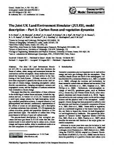
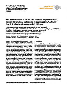
– Case 4: NE tree PFT killed by IFT 2, fate of DST based on black spruce (Picea mariana (Mill.) BSP) in eastern Canada (Angers et al., 2010); – Case 5: NE tree PFT killed by IFT 3, fate of DST based mostly on MPB-killed lodgepole pine (Pinus contorta var. latifolia) in western North America (Lewis and Hartley, 2005; Wulder et al., 2006; Griffin et al., 2011; Simard et al., 2011). The transfer of carbon from DST pools (i.e., fine roots, leaves/needles, and stems, the latter including coarse roots and branches) towards IBIS litter pools starts after a delay period and then occurs at a specific rate; note that the delay refers to the time of attack, even for Case 5. Table 2 gives the value of these parameters for the five cases currently implemented in MIM. In all cases, the DST fine roots are transferred to IBIS litter pools as a one-time event, at the end of the year of mortality (note that IBIS partitions all annual DST transfers into daily amounts over the following year). For deciduous PFTs (i.e., Cases 1 and 2), the transfer of DST leaves also occurs as a one-time event. On the other hand, the DST needles are transferred to litter pools over many years for evergreen PFTs (i.e., Cases 3–5). Finally, the DST stems are also transferred to litter pools over many years, usually starting after a 5-year delay period (see Fig. 1). As with the IFTrelated parameters, all these aspects of DST dynamics can easily be modified as a function of new data or to accommodate other tree species. Moreover, for large-scale studies, the IFT- and DST-related parameters could vary spatially to reflect within-species variation, instead of having uniform values as we have used here (e.g., needlefall for Case 5 could occur over more than 3 years). 3 3.1

Illustration of IBIS–MIM performance Simulation design

To illustrate the performance of IBIS–MIM, we conducted six simulations using the MPB-inspired IFT (i.e., IFT 3 from Table 1) with DST dynamics based mostly on MPB-killed lodgepole pine (i.e., Case 5 from Table 2). We performed an outbreak simulation and a control simulation in each of three different locations in British Columbia, Canada, henceforth designated as the northern, central, and southern grid cells (Table 3). These three locations, which we used as proxies to assess the influence of climate on the main outcomes, have suffered substantial MPB-caused mortality since 2000 (Walton, 2013). The mean annual temperature was almost equal in the northern and central grid cells, but summer was warmer and winter was colder in the former; the southern grid cell was warmer throughout the year. Annual precipitation was Geosci. Model Dev., 9, 1243–1261, 2016

1.0

Amount of DST stems (proportion of initial value)

– Case 3: NE tree PFT killed by IFT 2, fate of DST based on balsam fir (Abies balsamea (L.) Mill.) in eastern Canada (Angers et al., 2010);

0.9

Cases 1 and 5 Case 2 Case 3

0.8

Case 4

0.7

0.6

0.5

0.4

0.3

0.2

0.1

0.0 0

5

10

15

20

25

30

35

40

45

50

Time (years after mortality)

Figure 1. Litterfall schedule of DST stems for the five cases currently implemented in MIM (see Table 2). Mortality happened in year 0 and all values are for the end of the corresponding year.

very similar in the three grid cells, but summer rainfall was substantially lower in the southern grid cell, leading to lower soil water content during the growing season. All simulations started with the new 400-year spin-up procedure and were performed under a constant climate. In each grid cell, we prescribed a single 100 % mortality event happening in year 401 (i.e., in year 1 following the spin-up period) and continued the simulation up to year 1000. This single, 100 % mortality event does not aim to represent actual MPB outbreaks, but was implemented for the sake of simplicity, to increase the signal-to-noise ratio of the results, and to test the theoretical upper limit of impacts. We used the same climate data and weather generation for the outbreak simulation and the no-mortality control simulation performed in a given grid cell. In addition to yearly results throughout the entire simulation, we saved daily (monthly) results during 10 (200) years after the mortality event. We excluded the boreal BD tree PFT from simulations due to the generally low density of such trees within MPB-attacked stands in British Columbia (Hawkins et al., 2012). Consequently, competition took place among four different IBIS PFTs: boreal NE trees (i.e., the target PFT), evergreen shrubs, cold-deciduous shrubs, and C3 grasses. 3.2

Responses over different timescales

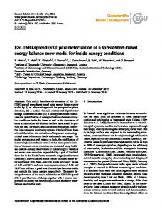
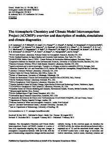
Figure 2 shows the effect of the single MPB outbreak on net primary productivity (NPP) in the three grid cells. In all cases, simulated NPP of the target NE trees decreased to zero while NPP of the lower canopy substantially increased following the 100 % mortality event; the productivity of the different PFTs then gradually resumed towards the pre-outbreak levels (Fig. 2a, c, and e). However, the growth release of the lower canopy was much stronger in the northern and central grid cells than in the southern grid cell, where condiwww.geosci-model-dev.net/9/1243/2016/

J.-S. Landry et al.: IBIS–MIM

1249

Table 2. Parameters for the dynamics of dead standing trees (DSTs) currently represented in MIM. Element

Case 1

Case 2

Case 3

Case 4

Case 5

Delay – fine roots Rate – fine roots Delay – leaves Rate – leavesc Delay – stems Rate – stemsc

Nonea

Nonea

Nonea

Nonea

One-timea

One-timea

One-timea

One-timea

Nonea,b One-timea,b 5 years 20 years

Nonea,b One-timea,b None 5 years (50 %) 10 years (50 %)

Noneb 3 yearsb 5 years 10 years (17 %) 10 years (83 %)

Noneb 3 yearsb 5 years 25 years (90 %) 15 years (10 %)

Nonea One-timea None 3 years 5 years 20 years

a All transferred to litter on the year of mortality. b If some leaves/needles remain because mortality occurred with less than 100 % defoliation or reflush happened. c Rates are linear and start after the delay period; for stems, some cases have two consecutive linear

periods showed on two lines: for each period, the duration (in years) and the total fraction transferred over the period (in %) are provided.

(a)

(b) 0.2

0.3

0.1

0.2

0.0 -0.1

0.1

∆NPP (kgC m-2 yr-1)

NPP (kgC m-2 yr-1)

0.4

-0.2 0.0 (c)

(d)

NE tree

Outbreak minus control 0.2

NPP (kgC m-2 yr-1)

Lower canopy 0.3

0.1

0.2

0.0 -0.1

0.1

∆NPP (kgC m-2 yr-1)

0.4

-0.2 0.0 (e)

(f) 0.2

0.3

0.1

0.2

0.0 -0.1

0.1

∆NPP (kgC m-2 yr-1)

NPP (kgC m-2 yr-1)

0.4

-0.2 0.0

0

100

200

300

400

500

600

Year

700

800

900

0

200

400

600

800

1000

Year

Figure 2. NPP results for an MPB outbreak (100 % mortality on year 401) simulated in IBIS–MIM: NPP of different PFTs (a, c, and e) and difference in total NPP with the control simulation (b, d, and f). NE is needleleaf evergreen; lower canopy is sum of evergreen shrubs, cold-deciduous shrubs, and C3 grasses. (a, b) Northern grid cell. (c, d) Central grid cell. (e, f) Southern grid cell.

tions were drier during the growing season. Such positive impacts on lower canopy have often been reported following outbreaks from MPB and other bark beetles (Stone and Wolfe, 1996; Klutsch et al., 2009; Griffin et al., 2011; Simard et al., 2011; Bowler et al., 2012; Brown et al., 2012; Vanderhoof et al., 2014). In the northern and central grid cells, the lower-canopy growth release exceeded the productivity losses coming from the death of NE trees, so that total post-outbreak NPP soon exceeded NPP in the control runs (Fig. 2b and d). The increase in 1NPP in the central grid cell from year ∼ 600 onwards came from the impact of the outbreak on the comwww.geosci-model-dev.net/9/1243/2016/

petition balance among PFTs: although NPP seemed relatively stable at the end of the spin-up (i.e., years 300–400 in Fig. 2c), lower-canopy NPP decreased markedly between years 600 and 750 in the control simulation, whereas the MPB outbreak released the lower canopy and postponed this decline, which seemed bound to happen in the long term. Empirical (Romme et al., 1986; Belovsky and Slade, 2000) and modelling (Mattson and Addy, 1975; Seidl et al., 2008; Albani et al., 2010; Pfeifer et al., 2011; Hansen, 2014) studies of insect damage have previously shown that total productivity, biomass, or carbon storage can be higher in disturbed than in undisturbed ecosystems. As was the case in IBIS– Geosci. Model Dev., 9, 1243–1261, 2016

1250

J.-S. Landry et al.: IBIS–MIM

Table 3. Input climate data and soil texture for the three grid cells. Element Coordinates (degrees) Latitude Longitude Temperature (◦ C) Annual Dec–Feb Mar–May Jun–Aug Sep–Nov Precipitation (mm day−1 ) Annual Dec–Feb Mar–May Jun–Aug Sep–Nov Soil texture Sand (%) Silt (%) Clay (%)

Northern

Central

Southern

55.25◦ N 123.75◦ W

52.75◦ N 124.75◦ W

49.75◦ N 120.25◦ W

+0.7 −11.3 +0.9 +11.9 +1.0

+0.8 −8.8 +0.4 +9.9 +1.4

+2.5 −6.8 +2.0 +12.0 +2.7

1.7 2.0 1.2 1.9 1.8 Sandy loam 65 25 10

1.6 1.9 1.1 1.6 1.7 Loam 42 40 18

1.6 2.3 1.4 1.3 1.6 Sandy loam 65 25 10

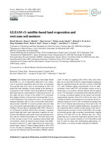
MIM, the mechanisms identified in these previous studies involved responses from non-target vegetation, i.e., other species or non-attacked age classes of the target species. In the southern grid cell, on the other hand, total NPP was reduced for about 75 years and then increased marginally for a few decades, before returning to the control level (Fig. 2f). The previous results also exhibited an interesting feature: in all grid cells, the recovery of the NE trees was initially very rapid, but was then reversed after ∼ 20–25 years before resuming again (Fig. 2a, c, and e). Although additional simulations would be required to confirm our hypothesis, we believe that this dip came from indirect biogeophysical interactions between recovering NE trees and decaying DSTs in the relatively cold climate considered here. After MPB mortality, the interception of radiation (shortwave and longwave) by DSTs warmed the surrounding air, allowing photosynthesis in the recovering NE trees to occur faster at a higher temperature than if DSTs had been absent. As DSTs gradually fell, NE trees captured more light but had a lower needle temperature, resulting in lower NPP. Such strong photosynthesis– temperature responses have been found to play a major role when simulating future vegetation dynamics (Sitch et al., 2008; Medvigy et al., 2010) and carbon cycle–climate feedbacks (Matthews et al., 2005). Figure 3 shows the impact of the outbreak on four variables (two related to carbon cycling, one to energy exchanges, and one to water cycling) over different timescales (yearly, monthly, and daily). The changes in net ecosystem productivity (NEP; Fig. 3a) were driven mostly by NPP, including the increases in total NPP ∼ 5 years post-mortality in the northern and central grid cells. Changes in heterotrophic respiration (Rh ) were generally smaller, but contributed to the NEP local minimum around year 25 (particularly visible in the central and southern grid cells) and progressively offset Geosci. Model Dev., 9, 1243–1261, 2016

the NPP increase in the northern and central grid cells, so that 1NEP became negligible after roughly a century. The total amount of aboveground litter (Fig. 3b) slightly decreased for a few years after the mortality event, because the total litterfall from DSTs in the outbreak simulations was initially lower than from live trees in the control simulations. After a few years, however, the situation was reversed and the increase in aboveground litter was > 1.5 kg C m−2 in all grid cells ∼ 25 years after the mortality event, gradually decreasing afterwards. After about 75 years, the aboveground litter was lower in the outbreak simulations due to the reduced litterfall from the still recovering vegetation. The pre-outbreak equilibrium was reached about 3 centuries after the mortality event. The monthly albedo (Fig. 3c) increased during the initial years as the needles fell from DSTs. The impact of snow cover was clearly apparent in the yearly cycle of albedo changes, with much higher albedo increases during winter months. The few points showing a decrease in albedo resulted from the earlier snowmelt in the outbreak simulations, a response that is illustrated for the central grid cell (Fig. 3d). While the snow amount was slightly higher following the first snowfall events (barely visible in Fig. 3d), in the middle of winter the control grid cells generally had more snow. But above all the snowmelt started and finished much earlier in the outbreak simulations, by about 3 weeks in the case illustrated. 3.3

Evaluation of performance

Table 4 presents a qualitative comparison of IBIS–MIM outcome after an MPB-caused 100 % mortality event with the results from 38 different studies based on field measurements, satellite data, or modelling. Except for some of the works reviewed in Mikkelson et al. (2013a), these studies all had actual control and effect results. Most studies assessed the impacts of mortality caused by MPB or other bark beetles, although a few studies depended upon other disturbances (girdling or clear cutting) for the effect. We note, however, that the identification of appropriate control stands for field and satellite studies is not a straightforward task, which may partly explain why the qualitative impact (increase, no change, or decrease) of MPB mortality varied across studies for some variables. Furthermore, the level of stand mortality differed among studies or was not quantified and, except for a few modelling studies, was less than the 100 % mortality simulated in IBIS–MIM. These limitations prevented us from performing more quantitative comparisons. The comparisons covered 28 different variables related to carbon cycling and vegetation dynamics, energy exchanges, and the water cycle. These comparisons further spanned various timescales: annual (all variables related to carbon cycling and vegetation dynamics, albedo, evapotranspiration, runoff, and soil moisture), seasonal/monthly (all variables related to energy exchanges, evapotranspiration, transpirawww.geosci-model-dev.net/9/1243/2016/

J.-S. Landry et al.: IBIS–MIM (a)

2.0 -2

∆litter–debris (kgC m )

∆NEP (kgC m-2 yr-1)

0.1

1251

0.0 -0.1 -0.2 Northern Central

-0.3

(b)

Northern Central

1.6

Southern

1.2 0.8 0.4 0.0

Southern

-0.4

-0.4 0

25

50

75

100

125

150

175

200

0

50

100

Time (years)

200

250

300

350

400

Time (years)

0.12

180 (c)

(d)

0.10

150

Snow amount (kg m )

∆albedo (unitless)

150

Control

-2

Northern 0.08

Central Southern

0.06 0.04 0.02

Outbreak 120 90 60 30

0.00 0 0

12

24

36

48

60

72

84

96

108

120

Time (months)

Aug 1

Nov 1

Feb 1

May 1

Time (days)

Figure 3. Impact of an MPB outbreak (100 % mortality) simulated in IBIS–MIM on different variables over various timescales. (a) Change (outbreak minus control) in NEP for the three grid cells; mortality happened on year 1. (b) Change (outbreak minus control) in aboveground litter (including coarse woody debris, but excluding dead standing trees) for the three grid cells; mortality happened on year 1. (c) Change (outbreak minus control) in albedo for the three grid cells; mortality happened on months 8 and 9 (August and September). (d) Snow amount in the central grid cell for the control and outbreak simulations; mortality happened 8 years before.

tion, soil moisture, snow depth/amount, and snowmelt onset), and daily (peak flow, snow depth/amount, and snowmelt onset). Among the 28 variables, IBIS–MIM prescribed only the snagfall dynamics of DSTs. IBIS–MIM results agreed with previous studies for most variables, thereby illustrating that the model constitutes an appropriate tool for studying the impacts of insect-induced plant damage on many interdependent variables spanning a large range of timescales. For most variables related to carbon cycling and vegetation dynamics, the qualitative responses of IBIS–MIM changed over time for two reasons. First, as seen in Sect. 3.2, lowercanopy biomass substantially increased following the canopy opening in the northern and central grid cells (but much less in the southern grid cell), eventually reversing the initial response for GPP, NPP, Ra , Rs , NEP, and total LAI (abbreviations are defined in Table 4) in these two locations ∼ 5– 15 years after the MPB outbreak. Note that the simulated increase in shrub biomass was marginal in the three grid cells, but that grass biomass increased substantially. Lower-canopy fractional cover increased in the northern grid cell only, because this variable was already at its maximum value before the mortality event in the other two grid cells. Second, the prescribed snagfall dynamics of DSTs led to a carbon response over multiple timescales (Edburg et al., 2011) that af-

www.geosci-model-dev.net/9/1243/2016/

fected Rh , NEP, and aboveground litter (see also Fig. 3a and b). Among the variables related to energy exchanges, IBIS– MIM responses for temperature and albedo systematically agreed with previous studies. (The air temperature in field studies was measured close to breast height, a level at which IBIS–MIM does not estimate temperature. As a proxy, we used the mean of the simulated temperature responses in the middle of the upper and lower canopies.) These responses became particularly strong and sustained after the complete fall of needles from DSTs. We note that the impacts on temperature variables in IBIS–MIM were generally opposite between winter and summer; unfortunately, none of the previous studies reported wintertime temperature changes. For latent and sensible heat fluxes, however, IBIS–MIM differed noticeably from previous studies: after the year of mortality, summertime latent heat flux actually increased for 3 years in the southern grid cell and for much longer in the other grid cells. The pattern was the opposite for summer sensible heat, except in the southern grid cell where this variable did not show a systematic behaviour. We think that these responses for summer turbulent heat fluxes had two different causes. For 1–4 years after the mortality event, the higher summer latent heat flux in all grid cells came from a ma-

Geosci. Model Dev., 9, 1243–1261, 2016

1252

J.-S. Landry et al.: IBIS–MIM

Table 4. Comparison of IBIS–MIM results for a simulated MPB outbreak with field-, satellite-, and model-based studies (increase: ↑; no change: –; decrease: ↓). Under the “field”, “satellite”, and “model” columns, the numbers refer to the studies listed below. Under the “IBIS– MIM” column, the values in parentheses give the number of grid cells sharing the same qualitative results (only provided when the three grid cells differed). Variable Gross primary productivity (GPP) Net primary productivity (NPP) Autotrophic respiration (Ra ) Heterotrophic respiration (Rh ) Soil respiration (Rs ) Net ecosystem productivity (NEP) Total or aboveground biomass Dead standing trees Aboveground litter–debris Total leaf area index (LAI) Canopy height Fractional cover, lower canopy Grass biomass Shrub biomass

Field

Satellite

Model

IBIS–MIM

↓1

↓3 ↓3,5 ↓3 ↑3 ↓3 ↓3 3,5,7 ↓ ↑3,7 ↑3,7,9 ↓3

↓a ↓a ↓a ↑c ↓a ↓a ↓ ↑ ↑c ↓a ↓ ↑(1) , –(2) ↑ ↑ (marginal)

↑1,14

↑15,16

↑ ↑

↑1,12,17,18 ↓14 ↑14

↓15 ↑15,19

↑ ↑ ↑ ↑(2);d , ↓(1);e –(1);e , ↓(2);d

↓1,14

↓16,19,20(1)

↑(2);d , ↓(1);e

Carbon cycle and vegetation dynamics ↓1,2 4;b ↓

Air temperature (T ), summer Land surface T , summer and month prior to snowfall Soil T , summer 1T surface vs. air, summer Albedo, seasons/annual Latent heat flux, summer Sensible heat flux, summer Evapotranspiration, summer/annual/n.s.f Transpiration, summer (first 2 years only) Runoff, annual/n.s.f Peak flow, n.s.f Soil moisture, seasons/annual/n.s.f Snow depth/amount, monthly/n.s.f Snowmelt onset, daily/monthly/n.s.f,i

–6 ↓6 ↑6 ↑8 , –6 ↓10 ↓8 11,12 ↑ , –6,9 8,9,13 ↑ ↑13 , –8,9 Energy exchanges ↑6,11 ↑11 ↑6,11 ↑8,11

Water cycle ↓20(1) ↓21

↓

↑20(4) , –20(1) ↑6,20(1) , –6 ↑20(3),22 , –20(2) ↑20(4),22 , –20(3) , ↓20(1)

↑16,19,20(2) ↑20(2) 16 ↑ , ↑ ↓19,g ↑16,19,20(1) ↑16,19,20(1)

↑a ↑ ↑h ↓ ↑

1 Bright et al. (2013); 2 Moore et al. (2013); 3 Edburg et al. (2011); 4 Romme et al. (1986); 5 Pfeifer et al. (2011); 6 Morehouse et al. (2008); 7 Caldwell et al. (2013); 8 Simard et al. (2011); 9 Klutsch et al. (2009); 10 Pugh and Gordon (2013); 11 Griffin et al. (2011); 12 Vanderhoof et al.

(2014); 13 Stone and Wolfe (1996); 14 Maness et al. (2013); 15 Wiedinmyer et al. (2012); 16 Mikkelson et al. (2013b); 17 O’Halloran et al. (2012); 18 Vanderhoof et al. (2013); 19 “LAI/4” case from Chen et al. (2015); 20 studies reviewed in Mikkelson et al. (2013a), the number of different studies being given in italics between parentheses; 21 Hubbard et al. (2013); 22 Pugh and Small (2012); a becomes the opposite after ∼ 5–15 years in the northern and central grid cells; b ↑ after 15–20 years in one out of four cases; c dominant response (high inter-annual variability); d except the first year, northern and central grid cells; e after 5 years, southern grid cell; f the time period for the studies reviewed in Mikkelson et al. (2013a) is not specified (n.s.), so comparisons with IBIS–MIM results were performed on an annual basis except for peak flow and snow-related variables (performed on a daily basis); g increase in spring and fall, decrease in summer; h for the first ∼ 5 years; i an increase means that snowmelt begins earlier in the year.

jor increase in evaporation, which, in turn, probably resulted from the combination of two pre-existing biases in the land surface module (LSX) that computes the exchanges of energy, water, and momentum within IBIS–MIM: (1) the overestimation of upper soil temperature in summer (El Maayar

Geosci. Model Dev., 9, 1243–1261, 2016

et al., 2001), which likely increased following the mortality event; and (2) the overestimation of heat storage within stems (including DSTs in our simulations), leading to an overestimated nighttime evaporation flux when the heat is released (Pollard and Thompson, 1995; El Maayar et al., 2001). For

www.geosci-model-dev.net/9/1243/2016/

J.-S. Landry et al.: IBIS–MIM ≥ 5 years after the mortality event, the increase in summer latent heat flux in the northern and central grid cells rather resulted from the strong growth of grasses mentioned previously. Indeed, NPP and LAI of grasses in these grid cells were then large enough to overcompensate for the decreases due to tree mortality, resulting in higher total transpiration, evapotranspiration, and latent heat flux. In the southern grid cell, where the response from grasses was much smaller, summer latent heat flux decreased ≥ 5 years post-mortality. While acknowledging possible issues with these IBIS– MIM results, particularly 1–4 years post-mortality, we want to underline the limitations from previous studies on turbulent heat fluxes and the closely related evapotranspiration. Three of the four modelling studies (Wiedinmyer et al., 2012; Mikkelson et al., 2013b; Chen et al., 2015) indirectly forced the responses they obtained by directly reducing the total canopy conductance without accounting for the possible growth release of the surviving vegetation, while the fourth modelling study (included in the Mikkelson et al., 2013a, review) only computed the change in runoff and then assumed no change in soil moisture to estimate the change in evapotranspiration. The two satellite-based studies rest upon the highly parameterized MODIS evapotranspiration data set (Mu et al., 2011), which has not been developed and tested in the context of MPB-killed forests. The only field-based study on evapotranspiration (included in the Mikkelson et al., 2013a, review) also neglected possible changes in soil moisture. Furthermore, other field-based studies – not included in our comparison due to their lack of control data – found very little change in evapotranspiration over various years following MPB mortality for sites located close to the northern grid cell (Bowler et al., 2012; Brown et al., 2014), or found that evapotranspiration increased over 3 years despite an ongoing increase in MPB mortality at a site in Wyoming, US (Reed et al., 2014). For water cycle variables besides evapotranspiration, the agreement with previous studies was also fairly good. The soil water budget in IBIS–MIM is very sensitive to the distribution of precipitation events during each month, so the responses were highly variable for runoff, peak flow, and soil moisture, particularly in the southern grid cell. Nevertheless, the responses provided in Table 4 were observed over the first ∼ 5 years. Afterwards, runoff remained higher in the outbreak simulation for the southern grid cell (resulting in part from the faster snowmelt), but became smaller in the other grid cells due to the increase in evapotranspiration as leaf area expanded. A field study on drought-induced tree mortality also linked an unexpected decrease in annual runoff to a growth release of the lower canopy (Guardiola-Claramonte et al., 2011). Peak flow, on the other hand, remained overall higher in all grid cells for at least a decade. After an initial increase lasting ∼ 5 years, soil moisture showed a sustained decrease, likely caused by the snowmelt-related higher runoff in the southern grid cell and by the higher evapotranspiration in the other grid cells. Although often slightly higher www.geosci-model-dev.net/9/1243/2016/

1253 at the beginning of the season, snow depth/amount overall decreased in IBIS–MIM (see Fig. 3d), contrary to most previous studies. This outcome likely resulted from the overestimated heat storage in DSTs and could lead to the simulated snow cover season ending too early. Yet areal snow coverage, which matters most for albedo, was equal for the control and outbreak simulations during most of the snow cover season and, most importantly, the earlier onset of snowmelt agreed with the majority of previous studies and was of reasonable magnitude. We checked whether the outcomes presented in Table 4 were sensitive or not to the specific weather simulated by performing two additional replicates for each grid cell. We found that the qualitative outcomes were the same for all variables, except for one minor difference: for one of the two replicates in the central grid cell, the post-outbreak fractional cover of the lower canopy increased slightly because it was not already at its maximum value, contrary to the case reported in Table 4. The quantitative results were also very similar across replicates, except for some water-related variables that are very sensitive to the exact timing of precipitation events. Finally, although assessing IBIS was not the point of this study and has already been done elsewhere (Foley et al., 1996; Delire and Foley, 1999; Kucharik et al., 2000, 2006; Lenters et al., 2000; El Maayar et al., 2001, 2002), the results obtained for the three grid cells compared favourably to recent studies, with a small underestimation of biomass (Beaudoin et al., 2014) and NPP (Gonsamo et al., 2013). Obtaining reliable data on soil carbon is notoriously difficult; when compared to the Harmonized World Soil Database (down to a depth of 1 m) as provided by Exbrayat et al. (2014), IBIS apparently overestimated soil carbon (down to a depth of 4 m), at least in the southern grid cell, even when accounting for the fact that a substantial fraction of soil carbon is found at a depth greater than 1 m (Jobbágy and Jackson, 2000).

4

Discussion

Many previous studies have represented insect damage in DVLSMs or less comprehensive climate-driven terrestrial models (Randerson et al., 1996; Krinner et al., 2005; Seidl et al., 2008; Wolf et al., 2008; Albani et al., 2010; Schäfer et al., 2010; Edburg et al., 2011; Medvigy et al., 2012; Mikkelson et al., 2013b; Chen et al., 2015). To our knowledge, however, our study is the first to assess, over daily to centennial timescales, the impacts from insect damage on vegetation dynamics and the carbon, energy, and water cycles in an integrated way (see Sect. 3). We compared the qualitative impacts of a simulated MPB outbreak on 28 IBIS–MIM variables with many field-, satellite-, and modelling-based studies (see Table 4), finding an overall good level of agreement. Our results further suggest that the physical presence of DSTs can benefit vegetation regrowth due to their interGeosci. Model Dev., 9, 1243–1261, 2016

1254 actions with radiation. A previous study also showed that falling DSTs can impact tree recovery through altered soil nitrogen dynamics (Edburg et al., 2011). Since DSTs contribute substantially to the biogeophysical and biogeochemical legacies of insect outbreaks, they should be explicitly modelled when feasible. We developed MIM to account for the major processes related to insect activity (Table 1), including the dynamics of DSTs (Table 2) when applicable. The generic design of the module could serve as a template to represent other IFTs and/or DSTs, and should facilitate future developments such as replacing the prescribed intra-annual unfolding of insect activity with algorithms based on simulated insect phenology. Moreover, MIM could be modified by simulating the fall of DSTs probabilistically (e.g., as in FireBGCv2; Keane et al., 2011) or enhanced by simulating the fall of DSTs as a function of environmental conditions (Lewis and Hartley, 2005) or the size of DSTs (e.g., as in FVS; Rebain et al., 2010), reducing snow albedo when needles fall from DSTs (Pugh and Small, 2012), and accounting for changes in needle optical properties as they turn from green to red (Wulder et al., 2006). The simple structure of MIM should also facilitate the adaptation of the module to other DVLSMs. Of course, MIM will then reflect many of the strengths and weaknesses of its host model. For example, the parameters of the boreal NE PFT in IBIS 2.6b4 were not based on lodgepole pine specifically. Furthermore, IBIS simulates a single boreal NE PFT, whereas different NE tree species can coexist in MPBattacked stands (Hawkins et al., 2012). Since IBIS does not represent different age cohorts within the same PFT, the model cannot account for the fact that MPB generally targets the larger trees (Axelson et al., 2009; Hawkins et al., 2012; Hansen, 2014). For < 100 % mortality, the responses of surviving younger trees would likely differ from those of surviving mature trees and could enhance the recovery of the target species. Impacts on tree demographics might also lead to complex stand-level responses, for example increasing total biomass despite reduced productivity because of a strong decrease in competition mortality (Pfeifer et al., 2011). Other shortcomings of IBIS that affected IBIS–MIM results came from the apparent overestimation of stem heat storage (Pollard and Thompson, 1995; El Maayar et al., 2001) and the absence of carbon–nutrient interactions (Edburg et al., 2011, 2012; Mikkelson et al., 2013a). On the other hand, IBIS twostrata vertical vegetation structure and detailed biophysics computations, both inherited directly from the LSX land surface module (Pollard and Thompson, 1995), allowed the lower-canopy growth release and the biogeophysical impacts of DSTs presence to be simulated more realistically than with many other DVLSMs. Finally, the strong link between climate and insect life cycles (Dukes et al., 2009; Bentz et al., 2010) provides an incentive for eventually enhancing MIM by including process-based representations of insect population dynamGeosci. Model Dev., 9, 1243–1261, 2016

J.-S. Landry et al.: IBIS–MIM ics in DVLSMs (Fosberg et al., 1999; Arneth and Niinemets, 2010), rather than prescribing insect damage through input data.

5

Conclusions

Insect damage to vegetation triggers major interacting effects on the cycles of carbon, nutrients, energy, and water, and also affects atmospheric chemistry. Given that dynamic vegetation–land surface models (DVLSMs) were designed to simulate coupled biogeophysical and biogeochemical fluxes within a consistent framework that accounts for changes in vegetation state, these models appear as good candidates to assess many of the consequences from insect-induced vegetation damage over a wide range of timescales. Here, we presented version 1.0 of the Marauding Insect Module (MIM) developed to simulate, within the Integrated BIosphere Simulator (IBIS) DVLSM, the impacts of prescribed levels of annual insect damage. MIM currently includes three insect functional types (IFTs) broadly representing defoliators of broadleaf trees, defoliators of needleleaf trees, and bark beetles. The parameterization of IFTs was based on key outbreaking insects affecting North American forests, but could be modified to represent other insect species, effects on other vegetation types (e.g., agricultural fields), and, with further adjustments, effects of some vegetation pathogens (e.g., Dietze and Matthes, 2014). Similarly, the fate of the insect-killed dead standing trees (DSTs) can easily be adjusted to go beyond the five cases currently implemented. Finally, MIM itself was designed in such a way that it should be transferable to other DVLSMs with limited adjustments. We also illustrated the realism and usefulness of IBIS– MIM by simulating a 100 % mortality event caused by the mountain pine beetle at three locations within British Columbia, Canada. First, we looked at the impacts of the outbreak on a variety of processes spanning daily to centennial timescales. One interesting outcome from this assessment is that DSTs intercept radiation and therefore warm the surrounding air, which in a cold climate could be beneficial for tree recovery. Second, we found that IBIS–MIM agreed qualitatively with the results from 38 field-, satellite-, and model-based studies for 28 different variables related to vegetation dynamics, and exchanges of carbon, energy, and water. These outcomes supported the idea that DVLSMs are valuable tools to study the consequences from insect-induced plant damage. Insect outbreaks, but also less spectacular backgroundlevel vegetation damage caused by insects, are part of the natural dynamics of terrestrial ecosystems worldwide. The use of IBIS–MIM and other similar process-based modelling tools suitable for climate-related studies should therefore help us better understand the wide range of possible impacts www.geosci-model-dev.net/9/1243/2016/

J.-S. Landry et al.: IBIS–MIM

1255

of insects on several processes in the Earth system, for past, current, and future conditions. Code availability The code for IBIS–MIM (in Fortran 77) is available upon request from the corresponding author or through the following link: http://landuse.geog.mcgill. ca/[email protected]/ibismim/. IBIS– MIM requires the NetCDF utilities (http://www.unidata.ucar. edu/software/netcdf/) for input and output data handling.

www.geosci-model-dev.net/9/1243/2016/

Geosci. Model Dev., 9, 1243–1261, 2016

1256

J.-S. Landry et al.: IBIS–MIM

Appendix A: Soil spin-up procedure

B2

The previous soil spin-up procedure lasted 150 years and was performed as follows: 40 iterations of the soil module were repeated each year during the first 75 years; then, during the following 25 years, the number of iterations per year decreased linearly from 40 to 1; and finally, during the last 50 years, soil carbon pools were brought to equilibrium under a single iteration per year. The total number of soil module iterations under this procedure was around 3500. The new soil spin-up procedure lasts 400 years and is performed as follows: 80 iterations of the soil module are repeated each year during the first 350 years; then, during the following 40 years, the number of iterations per year decreases linearly from 80 to 1; and finally, during the last 10 years, soil carbon pools are brought to equilibrium under a single iteration per year. The total number of soil module iterations under this procedure is around 29 600.

The total canopy photosynthesis (An,canopy , in mol CO2 s−1 m−2 of ground) is given by the following scaling integral:

Appendix B: Leaf-to-canopy scaling B1

The “extpar” simplification

The net photosynthesis (An (X), in mol CO2 s−1 m−2 of leaf) for a leaf that is X units into the upper or lower canopy (where X is the cumulative vegetation (leaf plus stem) area index, in m2 of vegetation m−2 of ground, with X = 0 at the top of the canopy) is computed as

Leaf-to-canopy scaling integral

LAI An,canopy = XAI

ZXAI An (X)dX,

(B4)

0

where LAI is the total canopy leaf area index and XAI is the total canopy vegetation (leaf plus stem) area index. Previously, the LAI/XAI factor was removed from the integral above and was included in the computation of the photosynthetically active radiation absorbed by leaves at the top of the canopy; the results for An,canopy were then the same for light-limiting conditions, but not under Rubisco-limiting or CO2 -limiting conditions. We therefore adjusted the code to work directly with Eq. (B4) under all conditions. Note that this adjustment and the removal of the extpar simplification affected canopy transpiration, which is computed as a function of canopy photosynthesis. Appendix C: Energy exchanges C1

Near-infrared optical properties of lower-canopy leaves

We modified the reflectance (unitless) from 0.60 to 0.40, and the transmittance (unitless) from 0.25 to 0.30.

An (X) = An (0)

A exp(−kX) + B exp(−hX) + C exp(hX) , A+B +C

(B1)

where An (0) is the photosynthesis for a leaf at the top of the canopy and A, B, C, k, and h are coefficients computed in IBIS. Previously, this expression was simplified to An (X) = An (0) exp(−extparX),

(B2)

C2

Snow albedo vs. solar zenith angle

IBIS increases snow albedo for solar zenith angles greater than 60◦ , but these increases appeared too large for very high zenith angles. We therefore limited these increases to a maximum of 10 % above the value at 60◦ for visible radiation and to a maximum of 15 % above the value at 60◦ for nearinfrared radiation.

with extpar =

Ak + Bh − Ch . A+B +C

C3 (B3)

Now, Eqs. (B2)–(B3) are not equal to Eq. (B1) unless kX and hX are both very small. We therefore worked directly with Eq. (B1) and removed the extpar simplification from the code. Note that this simplification might have been required in version 1 of IBIS, which used a different leaf-to-canopy scaling approach than version 2 (Foley et al., 1996; Kucharik et al., 2000).

Geosci. Model Dev., 9, 1243–1261, 2016

Visible and near-infrared snow albedo parameters

We decreased the following parameters related to snow albedo (unitless): low-temperature value in the visible (from 0.90 to 0.80), high-temperature value in the visible (from 0.70 to 0.60), low-temperature value in the near-infrared (from 0.60 to 0.50), and high-temperature value in the nearinfrared (from 0.40 to 0.30).

www.geosci-model-dev.net/9/1243/2016/

J.-S. Landry et al.: IBIS–MIM Author contributions. J.-S. Landry developed MIM and modified IBIS with advice from D. T. Price, N. Ramankutty, and L. Parrott; J.-S. Landry performed the simulations with IBIS–MIM and analyzed the results; J.-S. Landry prepared the manuscript with contributions from all co-authors.

Acknowledgements. We thank Barry Cooke, Ted Hogg, Jean-Noel Candau, Rich Fleming, and Jason Edwards (all from the Canadian Forest Service), as well as Andreas Fischlin (ETH Zürich) for advice on the Marauding Insect Module. We also thank the two reviewers for helping us improve the manuscript. J.-S. Landry was funded by a doctoral scholarship (B2) from the Fonds de recherche du Québec – Nature et technologies (FRQNT). Edited by: J. Kala

References Albani, M., Moorcroft, P. M., Ellison, A. M., Orwig, D. A., and Foster, D. R.: Predicting the impact of hemlock woolly adelgid on carbon dynamics of eastern United States forests, Can. J. Forest Res., 40, 119–133, 2010. Amiro, B. D., Barr, A. G., Barr, J. G., Black, T. A., Bracho, R., Brown, M., Chen, J., Clark, K. L., Davis, K. J., Desai, A. R., Dore, S., Engel, V., Fuentes, J. D., Goldstein, A. H., Goulden, M. L., Kolb, T. E., Lavigne, M. B., Law, B. E., Margolis, H. A., Martin, T., McCaughey, J. H., Misson, L., Montes-Helu, M., Noormets, A., Randerson, J. T., Starr, G., and Xiao, J.: Ecosystem carbon dioxide fluxes after disturbance in forests of North America, J. Geophys. Res., 115, G00K02, doi:10.1029/2010JG001390, 2010. Angers, V. A., Drapeau, P., and Bergeron, Y.: Snag degradation pathways of four North American boreal tree species, Forest Ecol. Manag., 259, 246–256, 2010. Arneth, A. and Niinemets, U.: Induced BVOCs: how to bug our models?, Trends Plant Sci., 15, 118–125, 2010. Axelson, J. N., Alfaro, R. I., and Hawkes, B. C.: Influence of fire and mountain pine beetle on the dynamics of lodgepole pine stands in British Columbia, Canada, Forest Ecol. Manag., 257, 1874– 1882, 2009. Barlage, M., Zeng, X., Wei, H., and Mitchell, K. E.: A global 0.05◦ maximum albedo dataset of snow-covered land based on MODIS observation, Geophys. Res. Lett., 32, L17405, doi:10.1029/2005GL022881, 2005. Beaudoin, A., Bernier, P. Y., Guindon, L., Villemaire, P., Guo, X. J., Stinson, G., Bergeron, T., Magnussen, S., and Hall, R. J.: Mapping attributes of Canada’s forests at moderate resolution through kNN and MODIS imagery, Can. J. Forest Res., 44, 521–532, 2014. Belovsky, G. E. and Slade, J. B.: Insect herbivory accelerates nutrient cycling and increases plant production, P. Natl. Acad. Sci. USA, 97, 14412–14417, 2000. Bentz, B. J., Régnière, J., Fettig, C. J., Hansen, E. M., Hayes, J. L., Hicke, J. A., Kelsey, R. G., Negrón, J. F., and Seybold, S. J.: Climate change and bark beetles of the Western United States and Canada: direct and indirect effects, Bioscience, 60, 602–613, 2010.

www.geosci-model-dev.net/9/1243/2016/

1257 Bowler, R., Fredeen, A. L., Brown, M., and Black, T. A.: Residual vegetation importance to net CO2 uptake in pinedominated stands following mountain pine beetle attack in British Columbia, Canada, Forest Ecol. Manag., 269, 82–91, 2012. Bright, B. C., Hicke, J. A., and Meddens, A. J. H.: Effects of bark beetle-caused tree mortality on biogeochemical and biogeophysical MODIS products, J. Geophys. Res.-Biogeo., 118, 974–982, 2013. Brown, M. G., Black, T. A., Nesic, Z., Fredeen, A. L., Foord, V. N., Spittlehouse, D. L., Bowler, R., Burton, P. J., Trofymow, J. A., Grant, N. J., and Lessard, D.: The carbon balance of two lodgepole pine stands recovering from mountain pine beetle attack in British Columbia, Agr. Forest Meteorol., 153, 82–93, 2012. Brown, M. G., Black, T. A., Nesic, Z., Foord, V. N., Spittlehouse, D. L., Freeden, A. L., Bowler, R., Grant, N. J., Burton, P. J., Trofymow, J. A., Lessard, D., and Meyer, G.: Evapotranspiration and canopy characteristics of two lodgepole pine stands following mountain pine beetle attack, Hydrol. Process., 28, 3326–3340, 2014. Caldwell, M. K., Hawbaker, T. J., Briggs, J. S., Cigan, P. W., and Stitt, S.: Simulated impacts of mountain pine beetle and wildfire disturbances on forest vegetation composition and carbon stocks in the Southern Rocky Mountains, Biogeosciences, 10, 8203– 8222, doi:10.5194/bg-10-8203-2013, 2013. Chen, F., Zhang, G., Barlage, M., Zhang, Y., Hicke, J. A., Meddens, A., Zhou, G., Massman, W. J., and Frank, J.: An observational and modeling study of impacts of bark beetle-caused tree mortality on surface energy and hydrological cycles, J. Hydrometeorol., 16, 744–761, 2015. Clark, K. L., Skowronski, N., and Hom, J.: Invasive insects impact forest carbon dynamics, Glob. Change Biol., 16, 88–101, 2010. Clark, K. L., Skowronski, N., Gallagher, M., Renninger, H., and Schäfer, K.: Effects of invasive insects and fire on forest energy exchange and evapotranspiration in the New Jersey pinelands, Agr. Forest Meteorol., 166–167, 50–61, 2012. Cook, B. D., Bolstad, P. V., Martin, J. G., Heinsch, F. A., Davis, J. K., Wang, W., Desai, A. R., and Teclaw, R. M.: Using light-use and production efficiency models to predict photosynthesis and net carbon exchange during forest canopy disturbance, Ecosystems, 11, 26–44, 2008. Cooke, B. J., Nealis, V. G., and Régnière, J.: Insect Defoliators as Periodic Disturbances in Northern Forest Ecosystems, in: Plant Disturbance Ecology, edited by: Johnson, E. A. and Mihanishi, K., Academic Press, 487–525, 2007. Couture, J. J. and Lindroth, R. L.: Atmospheric change alters performance of an invasive forest insect, Glob. Change Biol., 18, 3543–3557, 2012. Cramer, W., Bondeau, A., Woodward, F. I., Prentice, I. C., Betts, R. A., Brovkin, V., Cox, P. M., Fisher, V. A., Foley, J. A., Friend, A. D., Kucharik, C. J., Lomas, M. R., Ramankutty, N., Sitch, S., Smith, B., White, A., and Young-Molling, C.: Global response of terrestrial ecosystem structure and function to CO2 and climate change: results from six dynamic global vegetation models, Glob. Change Biol., 7, 357–373, 2001. Delire, C. and Foley, J. A.: Evaluating the performance of a land surface/ecosystem model with biophysical measurements from contrasting environments, J. Geophys. Res., 104, 16895–16909, 1999.

Geosci. Model Dev., 9, 1243–1261, 2016

1258 Dietze, M. C. and Matthes, J. H.: A general ecophysiological framework for modelling the impact of pests and pathogens on forest ecosystems, Ecol. Lett., 17, 1418–1426, 2014. Dukes, J. S., Pontius, J., Orwig, D., Garnas, J. R., Rodgers, V. L., Brazee, N., Cooke, B., Theoharides, K. A., Stange, E. E., Harrington, R., Ehrenfeld, J., Gurevitch, J., Lerdau, M., Stinson, K., Wick, R., and Ayres, M.: Responses of insect pests, pathogens, and invasive plant species to climate change in the forests of northeastern North America: What can we predict?, Can. J. Forest Res., 39, 231–248, 2009. Edburg, S. L., Hicke, J. A., Lawrence, D. M., and Thornton, P. E.: Simulating coupled carbon and nitrogen dynamics following mountain pine beetle outbreaks in the western United States, J. Geophys. Res., 116, G04033, doi:10.1029/2011JG001786, 2011. Edburg, S. L., Hicke, J. A., Brooks, P. D., Pendall, E. G., Ewers, B. E., Norton, U., Gochis, D., Gutmann, E. D., and Meddens, A. J. H.: Cascading impacts of bark beetle-caused tree mortality on coupled biogeophysical and biogeochemical processes, Front. Ecol. Environ., 10, 416–424, 2012. El Maayar, M., Price, D. T., Delire, C., Foley, J. A., Black, T. A., and Bessemoulin, P.: Validation of the integrated biosphere simulator over Canadian deciduous and coniferous boreal forest stands, J. Geophys. Res., 106, 14339–14355, 2001. El Maayar, M., Price, D. T., Black, T. A., Humphreys, E. R., and Jork, E.-M.: Sensitivity tests of the integrated biosphere simulator to soil and vegetation characteristics in a Pacific coastal coniferous forest, Atmos. Ocean, 40, 313–332, 2002. Exbrayat, J.-F., Pitman, A. J., and Abramowitz, G.: Disentangling residence time and temperature sensitivity of microbial decomposition in a global soil carbon model, Biogeosciences, 11, 6999–7008, doi:10.5194/bg-11-6999-2014, 2014. Fleming, R. A. and Volney, W. J. A.: Effects of climate change on insect defoliator population processes in Canada’s boreal forest: some plausible scenarios, Water Air Soil Poll., 82, 445–454, 1995. Foley, J. A., Prentice, I. C., Ramankutty, N., Levis, S., Pollard, D., Sitch, S., and Haxeltine, A.: An integrated biosphere model of land surface processes, terrestrial carbon balance, and vegetation dynamics, Global Biogeochem. Cy., 10, 603–628, 1996. Foley, J. A., Levis, S., Prentice, I. C., Pollard, D., and Thompson, S. L.: Coupling dynamic models of climate and vegetation, Glob. Change Biol., 4, 561–579, 1998. Fosberg, M. A., Cramer, W., Brovkin, V., Fleming, R., Gardner, R., Gill, A. M., Goldammer, J. G., Keane, R., Koehler, P., Lenihan, J., Neilson, R., Sitch, S., Thonicke, K., Venevsky, S., Weber, M. G., and Wittenberg, U.: Strategy for a fire module in dynamic global vegetation models, Int. J. Wildland Fire, 9, 79–84, 1999. Foster, J. R., Townsend, P. A., and Mladenoff, D. J.: Mapping asynchrony between gypsy moth egg-hatch and forest leaf-out: putting the phenological window hypothesis in a spatial context, Forest Ecol. Manag., 287, 67–76, 2013. Friedlingstein, P., Cox, P., Betts, R., Bopp, L., von Bloh, W., Brovkin, V., Cadule, P., Doney, S., Eby, M., Fung, I., Bala, G., John, J., Jones, C., Joos, F., Kato, T., Kawamiya, M., Knorr, W., Lindsay, K., Matthews, H. D., Raddatz, T., Rayner, P., Reick, C., Roeckner, E., Schnitzler, K.-G., Schnur, R., Strassmann, K., Weaver, A. J., Yoshikawa, C., and Zeng, N.: Climate–carbon cy-

Geosci. Model Dev., 9, 1243–1261, 2016

J.-S. Landry et al.: IBIS–MIM cle feedback analysis: results from the C4 MIP model intercomparison, J. Climate, 19, 3337–3353, 2006. Gonsamo, A., Chen, J. M., Price, D. T., Kurz, W. A., Liu, J., Boisvenue, C., Hember, R. A., Wu, C., and Chang, K.-H.: Improved assessment of gross and net primary productivity of Canada’s landmass, J. Geophys. Res.-Biogeo., 118, 1546–1560, 2013. Griffin, J. M., Turner, M. G., and Simard, M.: Nitrogen cycling following mountain pine beetle disturbance in lodgepole pine forests of Greater Yellowstone, Forest Ecol. Manag., 261, 1077– 1089, 2011. Guardiola-Claramonte, M., Troch, P. A., Breshears, D. D., Huxman, T. E., Switanek, M. B., Durcik, M., and Cobb, N. S.: Decreased streamflow in semi-arid basins following droughtinduced tree die off: a counter-intuitive and indirect climate impact on hydrology, J. Hydrol., 406, 225–233, 2011. Hansen, E. M.: Forest development and carbon dynamics after mountain pine beetle outbreaks, Forest Sci., 60, 476–488, 2014. Hawkins, C. D., Dhar, A., Balliet, N. A., and Runzer, K. D.: Residual mature trees and secondary stand structure after mountain pine beetle attack in central British Columbia, Forest Ecol. Manag., 277, 107–115, 2012. Hicke, J. A., Allen, C. D., Desai, A. R., Dietze, M. C., Hall, R. J., Hogg, E. H. T., Kashian, D. M., Moore, D., Raffa, K. F., Sturrock, R. N., and Vogelmann, J.: Effects of biotic disturbances on forest carbon cycling in the United States and Canada, Glob. Change Biol., 18, 7–34, 2012. Hogg, E. H. and Michaelian, M.: Factors affecting fall down rates of dead aspen (Populus tremuloides) biomass following severe drought in west-central Canada, Glob. Change Biol., 21, 1968– 1979, 2015. Hubbard, R. M., Rhoades, C. C., Elder, K., and Negron, J.: Changes in transpiration and foliage growth in lodgepole pine trees following mountain pine beetle attack and mechanical girdling, Forest Ecol. Manag., 289, 312–317, 2013. Hunter, M. D.: Insect population dynamics meets ecosystem ecology: effects of herbivory on soil nutrient dynamics, Agr. Forest Entomol., 3, 77–84, 2001. IBIS–MIM: available at: http://landuse.geog.mcgill.ca/ [email protected]/ibismim/, 2015. Jobbágy, E. G. and Jackson, R. B.: The vertical distribution of soil organic carbon and its relation to climate and vegetation, Ecol. Appl., 10, 423–436, 2000. Jones, B., Tardif, J., and Westwood, R.: Weekly xylem production in trembling aspen (Populus tremuloides) in response to artificial defoliation, Can. J. Botany, 82, 590–597, 2004. Keane, R. E., Loehman, R. A., and Holsinger, L. M.: The FireBGCv2 Landscape Fire Succession Model: A Research Simulation Platform for Exploring Fire and Vegetation Dynamics, USDA General Technical Report RMRS-GTR-255, 137 pp., United States Department of Agriculture, Forest Service, Rocky Mountain Research Station, Fort Collins, Colorado, USA, 2011. Klutsch, J. G., Negrón, J. F., Costello, S. L., Rhoades, C. C., West, D. R., Popp, J., and Caissie, R.: Stand characteristics and downed woody debris accumulations associated with a mountain pine beetle (Dendroctonus ponderosae Hopkins) outbreak in Colorado, Forest Ecol. Manag., 258, 641–649, 2009. Koller, C. N. and Leonard, D. E.: Comparison of energy budgets for spruce budworm Choristoneura fumiferana (Clemens) on balsam fir and white spruce, Oecologia, 49, 14–20, 1981.

www.geosci-model-dev.net/9/1243/2016/

J.-S. Landry et al.: IBIS–MIM Krinner, G., Viovy, N., de Noblet-Ducoudré, N., Ogée, J., Polcher, J., Friedlingstein, P., Ciais, P., Sitch, S., and Prentice, I. C.: A dynamic global vegetation model for studies of the coupled atmosphere-biosphere system, Global Biogeochem. Cy., 19, GB1015, doi:10.1029/2003GB002199, 2005. Kucharik, C. J., Foley, J. A., Delire, C., Fisher, V. A., Coe, M. T., Lenters, J. D., Young-Molling, C., Ramankutty, N., Norman, J. M., and Gower, S. T.: Testing the performance of a dynamic global ecosystem model: water balance, carbon balance, and vegetation structure, Global Biogeochem. Cy., 14, 795–825, 2000. Kucharik, C. J., Barford, C. C., El Maayar, M., Wofsy, S. C., Monson, R. K., and Baldocchi, D. D.: A multiyear evaluation of a dynamic global vegetation model at three AmeriFlux forest sites: vegetation structure, phenology, soil temperature, and CO2 and H2 O vapor exchange, Ecol. Model., 196, 1–31, 2006. Kurz, W. A., Dymond, C. C., Stinson, G., Rampley, G. J., Neilson, E. T., Carroll, A. L., Ebata, T., and Safranyik, L.: Mountain pine beetle and forest carbon feedback to climate change, Nature, 452, 987–990, 2008. Landry, J.-S. and Parrott, L.: Could the lateral transfer of nutrients by outbreaking insects lead to consequential landscape-scale effects?, Ecosphere, 7, e01265, doi:10.1002/ecs2.1265, 2016. Landsberg, J. and Ohmart, C.: Levels of insect defoliation in forests: patterns and concepts, Trends Ecol. Evol., 4, 96–100, 1989. Lenters, J. D., Coe, M. T., and Foley, J. A.: Surface water balance of the continental United States, 1963–1995: regional evaluation of a terrestrial biosphere model and the NCEP/NCAR reanalysis, J. Geophys. Res., 105, 22393–22425, 2000. Lewis, K. J. and Hartley, I.: Rate of deterioration, degrade and fall of trees killed by mountain pine beetle: a synthesis of the literature and experiential knowledge, Mountain Pine Beetle Initiative Working Paper 2005–14, Canadian Forest Service, Pacific Forestry Centre, Victoria, British Columbia, 27 pp., 2005. Lovett, G. M., Christenson, L. M., Groffman, P. M., Jones, C. G., Hart, J. E., and Mitchell, M. J.: Insect defoliation and nitrogen cycling in forests, Bioscience, 52, 335–341, 2002. Maness, H., Kushner, P. J., and Fung, I.: Summertime climate response to mountain pine beetle disturbance in British Columbia, Nat. Geosci., 6, 65–70, 2013. Matthews, H. D., Eby, M., Weaver, A. J., and Hawkins, B. J.: Primary productivity control of simulated carbon cycle– climate feedbacks, Geophys. Res. Lett., 32, L14708, doi:10.1029/2005GL022941, 2005. Mattson, W. J. and Addy, N. D.: Phytophagous insects as regulators of forest primary production, Science, 190, 515–522, 1975. McGuire, A. D., Sitch, S., Clein, J. S., Dargaville, R., Esser, G., Foley, J. A., Heimann, M., Joos, F., Kaplan, J., Kicklighter, D. W., Meier, R. A., Melillo, J. M., Moore III, B., Prentice, I. C., Ramankutty, N., Reichenau, T., Schloss, A., Tian, H., Williams, L. J., and Wittenberg, U.: Carbon balance of the terrestrial biosphere in the twentieth century: analyses of CO2 , climate and land use effects with four process-based ecosystem models, Global Biogeochem. Cy., 15, 183–206, 2001. McNaughton, S. J., Oesterheld, M., Frank, D. A., and Williams, K. J.: Ecosystem-level patterns of primary productivity and herbivory in terrestrial habitats, Nature, 341, 142–144, 1989.

www.geosci-model-dev.net/9/1243/2016/

1259 Medvigy, D., Wofsy, S. C., Munger, J. W., and Moorcroft, P. R.: Responses of terrestrial ecosystems and carbon budgets to current and future environmental variability, P. Natl. Acad. Sci. USA, 107, 8275–8280, 2010. Medvigy, D., Clark, K. L., Skowronski, N. S., and Schäfer, K. V. R.: Simulated impacts of insect defoliation on forest carbon dynamics, Environ. Res. Lett., 7, 045703, doi:10.1088/17489326/7/4/045703, 2012. Metcalfe, D. B., Asner, G. P., Martin, R. E., Silva Espejo, J. E., Huasco, W. H., Farfán Amézquita, F. F., Carranza-Jimenez, L., Galiano Cabrera, D. F., Baca, L. D., Sinca, F., Huaraca Quispe, L. P., Taype, I. A., Mora, L. E., Dávila, A. R., Solórzano, M. M., Puma Vilca, B. L., Laupa Román, J. M., Guerra Bustios, P. C., Revilla, N. S., Tupayachi, R., Girardin, C. A. J., Doughty, C. E., and Malhi, Y.: Herbivory makes major contributions to ecosystem carbon and nutrient cycling in tropical forests, Ecol. Lett., 17, 324–332, 2014. Mikkelson, K. M., Bearup, L. A., Maxwell, R. M., Stednick, J. D., McCray, J. E., and Sharp, J. O.: Bark beetle infestation impacts on nutrient cycling, water quality and interdependent hydrological effects, Biogeochemistry, 115, 1–21, 2013a. Mikkelson, K. M., Maxwell, R. M., Ferguson, I., Stednick, J. D., McCray, J. E., and Sharp, J. O.: Mountain pine beetle infestation impacts: modeling water and energy budgets at the hill-slope scale, Ecohydrology, 6, 64–72, 2013b. Moore, D. J. P., Trahan, N. A., Wilkes, P., Quaife, T., Stephens, B. B., Elder, K., Desai, A. R., Negron, J., and Monson, R. K.: Persistent reduced ecosystem respiration after insect disturbance in high elevation forests, Ecol. Lett., 16, 731–737, 2013. Morehouse, K., Johns, T., Kaye, J., and Kaye, M.: Carbon and nitrogen cycling immediately following bark beetle outbreaks in southwestern ponderosa pine forests, Forest Ecol. Manag., 255, 2698–2708, 2008. Mu, Q., Zhao, M., and Running, S. W.: Improvements to a MODIS global terrestrial evapotranspiration algorithm, Remote Sens. Environ., 115, 1781–1800, 2011. NetCDF utilities: available at: http://www.unidata.ucar.edu/ software/netcdf/, 2016. New, M., Hulme, M., and Jones, P.: Representing twentieth-century space–time climate variability. Part I: Development of a 1961– 1990 mean monthly terrestrial climatology, J. Climate, 12, 829– 856, 1999. NRCan: Trees, insects and diseases of Canada’s forests, Forest tent caterpillar, Natural Resources Canada, available at: http: //tidcf.nrcan.gc.ca/en/insects/factsheet/9374 (last access: 28 January 2013), 2012. O’Halloran, T. L., Law, B. E., Goulden, M. L., Wang, Z., Barr, J. G., Schaaf, C., Brown, M., Fuentes, J. D., Göckede, M., Black, A., and Engel, V.: Radiative forcing of natural forest disturbances, Glob. Change Biol., 18, 555–565, 2012. Oleson, K. W., Lawrence, D. M., Bonan, G. B., Flanner, M. G., Kluzek, E., Lawrence, P. J., Levis, S., Swenson, S. C., Thornton, P. E., Dai, A., Decker, M., Dickinson, R., Feddema, J., Heald, C. L., Hoffman, F., Lamarque, J.-F., Mahowald, N., Niu, G.-Y., Qian, T., Randerson, J., Running, S., Sakaguchi, K., Slater, A., Stöckli, R., Wang, A., Yang, Z.-L., Zeng, X., and Zeng, X.: Technical Description of version 4.0 of the Community Land Model (CLM), NCAR Technical Note NCAR/TN-

Geosci. Model Dev., 9, 1243–1261, 2016

1260 478+STR, 257 pp., National Center for Atmospheric Research, Boulder, Colorado, USA, 2010. Pfeifer, E. M., Hicke, J. A., and Meddens, A. J. H.: Observations and modeling of aboveground tree carbon stocks and fluxes following a bark beetle outbreak in the western United States, Glob. Change Biol., 17, 339–350, 2011. Pollard, D. and Thompson, S. L.: Use of a land-surface-transfer scheme (LSX) in a global climate model: the response to doubling stomatal resistance, Global Planet. Change, 10, 129–161, 1995. Prentice, I. C., Bondeau, A., Cramer, W., Harrison, S. P., Hickler, T., Lucht, W., Sitch, S., Smith, B., and Sykes, M. T.: Dynamic global vegetation modeling: quantifying terrestrial ecosystem responses to large-scale environmental change, in: Terrestrial Ecosystems in a Changing World, edited by: Canadell, J. G., Pataki, D. E., and Pitelka, L. F., Springer, 175–192, 2007. Pugh, E. and Gordon, E.: A conceptual model of water yield effects from beetle-induced tree death in snow-dominated lodgepole pine forests, Hydrol. Process., 27, 2048–2060, 2013. Pugh, E. and Small, E.: The impact of pine beetle infestation on snow accumulation and melt in the headwaters of the Colorado River, Ecohydrology, 5, 467–477, 2012. Quillet, A., Peng, C., and Garneau, M.: Toward dynamic global vegetation models for simulating vegetation-climate interactions and feedbacks: recent developments, limitations, and future challenges, Environ. Rev., 18, 333–353, 2010. Randerson, J. T., Thompson, M. V., Malmstrom, C. M., Field, C. B., and Fung, I. Y.: Substrate limitations for heterotrophs: implications for models that estimate the seasonal cycle of atmospheric CO2 , Global Biogeochem. Cy., 10, 585–602, 1996. Rebain, S. A., Reinhard, E. D., Crookston, N. L., Beukema, S. J., Kurz, W. A., Greenough, J. A., Robinson, D, C. E., and Lutes, D. C.: The Fire and Fuels Extension to the Forest Vegetation Simulator: Updated Model Documentation, 403 pp., Internal Report, United States Department of Agriculture, Forest Service, Forest Management Service Center, Fort Collins, Colorado, USA, 2010 (revised 2015). Reed, D. E., Ewers, B. E., and Pendall, E.: Impact of mountain pine beetle induced mortality on forest carbon and water fluxes, Environ. Res. Lett., 9, 105004, doi:10.1088/1748-9326/9/10/105004, 2014. Régnière, J. and You, M.: A simulation model of spruce budworm (Lepidoptera: Tortricidae) feeding on balsam fir and white spruce, Ecol. Model., 54, 277–297, 1991. Romme, W. H., Knight, D. H., and Yavitt, J. B.: Mountain pine beetle outbreaks in the Rocky Mountains: regulators of primary productivity?, Am. Nat., 127, 484–494, 1986. Royama, T.: Population dynamics of the spruce budworm Choristoneura Fumiferana, Ecol. Monogr., 54, 429–462, 1984. Royama, T., MacKinnon, W. E., Kettela, E. G., Carter, N. E., and Hartling, L. K.: Analysis of spruce budworm outbreak cycles in New Brunswick, Canada, since 1952, Ecology, 86, 1212–1224, 2005. Safranyik, L. and Carroll, A. L.: The biology and epidemiology of the mountain pine beetle in lodgepole pine forests, in: The Mountain Pine Beetle: A Synthesis of Biology, Management, and Impacts on Lodgepole Pine, edited by: Safranyik, L. and Wilson, B., Natural Resources Canada, Victoria, Canada, 3–66, 2006.

Geosci. Model Dev., 9, 1243–1261, 2016

J.-S. Landry et al.: IBIS–MIM Schäfer, K. V. R., Clark, K. L., Skowronski, N., and Hamerlynck, E. P.: Impact of insect defoliation on forest carbon balance as assessed with a canopy assimilation model, Glob. Change Biol., 16, 546–560, 2010. Seidl, R., Rammer, W., Jäger, D., and Lexer, M. J.: Impact of bark beetle (Ips typographus L.) disturbance on timber production and carbon sequestration in different management strategies under climate change, Forest Ecol. Manag., 256, 209–220, 2008. Seidl, R., Schelhaas, M.-J., Rammer, W., and Verkerk, P. J.: Increasing forest disturbances in Europe and their impact on carbon storage, Nat. Clim. Change, 4, 806–810, 2014. Simard, M., Romme, W. H., Griffin, J. M., and Turner, M. G.: Do mountain pine beetle outbreaks change the probability of active crown fire in lodgepole pine forests?, Ecol. Monogr., 81, 3–24, 2011. Sitch, S., Huntingford, C., Gedney, N., Levy, P. E., Lomas, M., Piao, S. L., Betts, R., Ciais, P., Cox, P., Friedlingstein, P., Jones, C. D., Prentice, I. C., and Woodward, F. I.: Evaluation of the terrestrial carbon cycle, future plant geography and climatecarbon cycle feedbacks using five Dynamic Global Vegetation Models (DGVMs), Glob. Change Biol., 14, 2015–2039, 2008. Stinson, G., Kurz, W. A., Smyth, C. E., Neilson, E. T., Dymond, C. C., Metsaranta, J. M., Boisvenue, C., Rampley, G. J., Li, Q., White, T. M., and Blain, D.: An inventory-based analysis of Canada’s managed forest carbon dynamics, 1990 to 2008, Glob. Change Biol., 17, 2227–2244, 2011. Stone, W. E. and Wolfe, M. L.: Responses of understory vegetation to variable tree mortality following a mountain pine beetle epidemic in lodgepole pine stands in northern Utah, Vegetatio, 122, 1–12, 1996. Turcotte, M. M., Thomsen, C. J. M., Broadhead, G. T., Fine, P. V. A., Godfrey, R. M., Lamarre, G. P. A., Meyer, S. T., Richards, L. A., and Johnson, M. T. J.: Percentage leaf herbivory across vascular plant species, Ecology, 95, 788, doi:10.1890/131741.1, 2014. Vanderhoof, M., Williams, C. A., Ghimire, B., and Rogan, J.: Impact of mountain pine beetle outbreaks on forest albedo and radiative forcing, as derived from Moderate Resolution Imaging Spectroradiometer, Rocky Mountains, USA, J. Geophys. Res.Biogeo., 118, 1461–1471, 2013. Vanderhoof, M., Williams, C. A., Shuai, Y., Jarvis, D., Kulakowski, D., and Masek, J.: Albedo-induced radiative forcing from mountain pine beetle outbreaks in forests, south-central Rocky Mountains: magnitude, persistence, and relation to outbreak severity, Biogeosciences, 11, 563–575, doi:10.5194/bg-11-563-2014, 2014. Walton, A.: Provincial-Level Projection of the Current Mountain Pine Beetle Outbreak: Update of the Infestation Projection Based on the Provincial Aerial Overview Surveys of Forest Health conducted from 1999 through 2012 and the BCMPB model (year 10), BC Forest Service, 2013. Wang, Z. and Zeng, X.: Snow albedo’s dependence on Solar zenith angle from in situ and MODIS data, Atmospheric and Oceanic Science Letters, 1, 45–50, 2008. Wiedinmyer, C., Barlage, M., Tewari, M., and Chen, F.: Meteorological impacts of forest mortality due to insect infestation in Colorado, Earth Interact., 16, 1–11, 2012. Wolf, A., Kozlov, M. V., and Callaghan, T. V.: Impact of nonoutbreak insect damage on vegetation in northern Europe will

www.geosci-model-dev.net/9/1243/2016/

J.-S. Landry et al.: IBIS–MIM be greater than expected during a changing climate, Climatic Change, 87, 91–106, 2008. Wulder, M. A., Dymond, C. C., White, J. C., Leckie, D. G., and Carroll, A. L.: Surveying mountain pine beetle damage of forests: a review of remote sensing opportunities, Forest Ecol. Manag., 221, 27–41, 2006.

www.geosci-model-dev.net/9/1243/2016/

1261 Yang, L. E.: The ecological consequences of insect outbreaks, in: Insect Outbreaks Revisited, edited by: Barbosa, P., Letourneau, D. K., and Agrawal, A. A., Blackwell Publishing, 197– 218, Chichester, West Sussex, UK, 2012.

Geosci. Model Dev., 9, 1243–1261, 2016