a robot manipulator to reach a target point in its workspace using visual feedback. This involves primarily two tasks na
Implementation of a neural network based visual motor control algorithm for a 7 DOF redundant manipulator Swagat Kumar and Laxmidhar Behera
Abstract— This paper deals with visual-motor coordination of a 7 dof robot manipulator for pick and place applications. Three issues are dealt with in this paper - finding a feasible inverse kinematic solution without using any orientation information, resolving redundancy at position level and finally maintaining the fidelity of information during clustering process thereby increasing accuracy of inverse kinematic solution. A 3dimensional KSOM lattice is used to locally linearize the inverse kinematic relationship. The joint angle vector is divided into two groups and their effect on end-effector position is decoupled using a concept called function decomposition. It is shown that function decomposition leads to significant improvement in accuracy of inverse kinematic solution. However, this method yields a unique inverse kinematic solution for a given target point. A concept called sub-clustering in configuration space is suggested to preserve redundancy during learning process and redundancy is resolved at position level using several criteria. Even though the training is carried out off-line, the trained network is used online to compute the required joint angle vector in only one step. The accuracy attained is better than the current state of art. The experiment is implemented in real-time and the results are found to corroborate theoretical findings.
I. I NTRODUCTION Visual motor coordination or control is the task of guiding a robot manipulator to reach a target point in its workspace using visual feedback. This involves primarily two tasks namely, extracting the coordinate information of robot endeffector and target point from camera images and then finding out necessary joint angle movement to reach the target point. The first task involves camera calibration to find out an approximate model of the camera so that a mapping from pixel coordinates to real world coordinates is obtained. Tsai’s algorithm [1] is one of the most widely used method for this purpose. The second task is more commonly known as solving inverse kinematic problem. Robots with seven or more degrees of freedom (DOF) are kinematically redundant, since six joints are sufficient for arbitrary end-effector placement (including position and orientation). Although the availability of ’extra’ joints can provide dexterous motion of the arm, proper utilization of this redundancy poses a challenging and difficult problem [2]. The extra degrees of freedom may be used to meet the joint angle limits, avoid obstacles as well as kinematic singularity or optimize additional constraints like manipulability or force The authors are with the Department of Electrical Engineering, Indian Institute of Technology Kanpur, Uttar Pradesh, India (email: {swagatk,lbehera}@iitk.ac.in). This work was supported by Department of Science and Technology (DST), Govt. of India under FIST grant for intelligent control and sensor laboratory
constraints. A number of techniques have been proposed in literature to resolve redundancy [3], [2], [4], [5]. However, most of these techniques resolve redundancy at velocity or acceleration level. Use of neural networks to solve inverse kinematic problem in visual motor control paradigm is quite old. Kohonen’s self organizing map [6] (KSOM) based neural architectures have been found to be useful for solving inverse kinematic problems for 3 dof manipulators [7], [8], [9]. Parametrized self organizing maps (PSOM) [10] have been used by many researchers for solving inverse kinematic problem of manipulators with higher degrees of freedom [11], [12]. However, redundancy resolution at position level has not been considered explicitly in these works. This paper is concerned with finding a feasible inverse kinematic solution of a 7 dof robot manipulator for pick and place application. The purpose is to find a feasible joint angle vector directly from the end-effector position. Since several such joint angle vectors may give rise to same end-effector position, the problem necessitates resolving redundancy as well. This is in contrast with most of the current methods where the orientation information is used explicitly for solving inverse kinematics. In this paper, a 3-dimensional KSOM lattice is used to discretize the input space. Each node in the KSOM lattice represents a distinct point in the input space. Using Taylor series expansion, the inverse kinematic relationship is linearized around these points. The computation of necessary joint angle vector for a given end-effector position requires the knowledge of inverse of Jacobian matrices at each such points. Since only the position information is used for computing the joint angle vector, the Jacobean matrix turns out to be a non-invertible rectangular matrix. To improve the tracking accuracy, the joint angle vector is divided into two groups and the effect of each group on the end-effector position is decoupled from the other using a function decomposition scheme. This method however gives rise to only one feasible joint angle vector for a given target position. Three degrees of freedom are enough for reaching a point in a 3-dimensional workspace. Extra degrees of freedom provide dexterity in the sense that the same task may be performed with several different joint angle combinations. The number of available configurations for a given end-effector position may be infinite. It is pertinent to reduce the number of such available solutions to a manageable finite number and then selecting a configuration that best suits the task at hand. With this objective, various sub-clusters are created in the joint angle
space corresponding to each neuron in the Cartesian space. In these two methods, the inverse Jacobian matrices are computed directly from the training data using least square technique. However, these two matrices may also be learned incrementally using a gradient-descent algorithm. It is a well known fact that any kind of clustering introduces noise into information. Hence, the significance of preserving the fidelity of data in learning based methods and its effect on inverse kinematic solution is analyzed. The proposed methods are implemented in real-time on a 7DOF PowerCube™ manipulator from Amtec Robotics [13]. Following section describes the system model for visual motor coordination. KSOM based inverse kinematic solution is explained in section III. Various issues related to clustering are discussed in section IV. The function decomposition based scheme for inverse kinematic solution is described in section V. Redundancy resolution using sub-clustering in joint angle space is considered in section VI. The simulation and experimental results are provided in section VII followed by conclusion in section VIII. II. S YSTEM M ODEL A. Experimental Setup The schematic of visual-motor control setup is shown in Figure 1. It consists of a stereo-camera system, a robot manipulator and processing unit for running algorithm. Image processing part is used to extract 4 dimensional image coordinate vectors for current robot position (Pr ) and target point (Pt ) to be reached in the workspace. The Neural network module computes the necessary joint angle vector θ, which in turn drives the robot manipulator through a jointservo module. Pt Neural Network
Pr
Image Processing Unit
Joint angle vector
(u1 , u2 ) (u3 , u4 )
Camera1
Camera2
θ Target Servo Driving Unit 7DOF PowerCube Robot Manipulator
Fig. 1.
Schematic of Visual Motor Coordination
B. The Manipulator Model We use a 7DOF PowerCube™ robot manipulator [13] for experimentation. The model of the manipulator is derived from its link geometry. The D-H parameters are used to derive forward kinematic equations for the manipulator. The
end-effector position is given by following equations: x
= (−(((c1 c2 c3 − s1 s3 )c4 − c1 s2 s4 )c5 + (−c1 c2 s3 − s1 c3 )s5 )s6 + (−(c1 c2 c3 − s1 s3 )s4 − c1 s2 c4 )c6 )d7 + (−(c1 c2 c3 − s1 s3 )s4 − c1 s2 c4 )d5 − c1 s2 d3
y
= (−(((s1 c2 c3 + c1 s3 )c4 − s1 s2 s4 )c5 + (−s1 c2 s3 + c1 c3 )s5 )s6 + (−(s1 c2 c3 + c1 s3 )s4 − s1 s2 c4 )c6 )d7 + (−(s1 c2 c3 + c1 s3 )s4 − s1 s2 c4 )d5 − s1 s2 d3
z
= (−((s2 c3 c4 + c2 s4 )c5 − s2 s3 s5 )s6 + (−s2 c3 s4 + c2 c4 )c6 )d7 + (−s2 c3 s4 + c2 c4 )d5 + c2 d3 + d1
(1)
where various parameters are : d1 = 0.390 m, d3 = 0.370 m, d5 = 0.310 m, d7 = 0.2656 m, ci = cos θi , si = sin θi , i = 1, 2, . . . 6. Note that the end-effector position [x y z]′ does not depend on the seventh joint angle. However, the techniques provided in this paper are applicable to any number of joints. C. The Camera Model The tip of robot end-effector is viewed through a stereo camera system. In order to derive the forward kinematic model between joint angle vectors and image coordinates of end-effector, we need to convert the Cartesian coordinate of end-effector into its corresponding pixel coordinates in the image plane. This necessitates a camera model. Camera calibration consists of estimating model parameters for an un-calibrated camera. Tsai’s algorithm [1] for noncoplanar camera calibration is used to estimate 11 parameters - extrinsic (Rx , Ry , Rz , Tx , Ty , Tz ) and intrinsic (f, κ, Cx , Cy , sx ). The relationship between the position of a point P in world coordinates (xw , yw , zw ) and the point’s image in the camera’s frame buffer (xf , yf ) is defined by a sequence of coordinate transformations. The image coordinate of point P is given by sx xd xf = + Cx dx yd + Cy (2) yf = dy where sx is the scaling factor, dx and dy are the x and y dimensions of camera’s sensor element respectively, Cx , Cy are pixels coordinates of image center and xd and yd are true position on image plane considering radial distortions. The detailed derivation of these equations are available in [1] and [9]. D. The Problem Definition The forward map between 7-dimensional joint angle space to 4-dimensional image coordinate space is obtained by using
manipulator forward kinematic model (1) and camera model (2). This forward mapping may be represented as u = f (θ)
(3)
where u is the 4-dimensional image coordinate vector obtained from two cameras and θ is the 7-dimensional joint angle vector. The task is to compute the necessary joint angle vector for a target point ut . The inverse kinematic problem is given by θ = f −1 (ut ) = r(ut ) (4) This inverse kinematic problem is ill-posed and may have infinte number of solutions. Following issues are addressed in this paper: • Inverse Kinematic solution: Inverse kinematics is solved without using orientation information. • Redundancy Resolution: Since a target position may be associated with several joint angle vectors, one needs to choose from several such available solutions. • Improving the accuracy in reaching the target point by preserving the fidelity of information available in training data. III. I NVERSE K INEMATIC S OLUTION OF M ANIPULATOR USING KSOM
A
7 DOF
As mentioned above, the inverse kinematic relationship (4) is a one-to-many mapping and hence difficult to learn. One popular approach to this problem involves discretizing input as well as output spaces into several small cells so that a linear map from input to output space holds good within each cell. The linear inverse kinematic relationship for each region is obtained using Taylor series expansion as shown below: ∂r θ − θ0 = (x − x0 ) (5) ∂x (x0 ,θ0 ) where (x0 , θ0 ) is the centre of the cell, x is the target point lying within this cell and θ is the joint angle vector needed for reaching this target point. ∂r For a sufficiently small region, the Jacobian matrix ∂x may be approximated with a constant matrix D0 . Hence, each cell is associated with a 4-dimensional x0 vector, a 7-dimensional θ0 vector and a 7×4 dimensional Jacobian matrix D0 and the inverse kinematic relationship for this cell may be rewritten as θ − θ0 = D0 (x − x0 ) (6) Once the inverse Jacobian matrix D0 is learnt, the required joint angle is computed in a single step without using any orientation information at the target point. In our case, the last joint angle θ7 does not contribute to end-effector position and hence without any loss of generality, we consider the joint angle vector θ to have a dimension 6 × 1. Finding a feasible joint angle vector for a given end-effector position without using orientation information is useful in case of visual motor coordination where it might be expensive to extract orientation information from camera images.
A 3 dimensional KSOM lattice is used to discretize the input and output spaces. Lattice node indices are represented by γ and each such node is associated with a weight vector wγ of dimension 4 × 1, a joint angle vector θ γ of dimension 6 × 1 and an inverse Jacobian matrix Dγ of dimension 6 × 4. The vector wγ discretizes the input space and θγ discretizes the output space. Since for every wγ , we have only one joint angle vector θ γ associated with it, this method gives only one inverse kinematic solution even for a redundant manipulator. Computation of inverse Jacobian matrix Once the input and output spaces are discretized using KSOM lattice, collect all data pairs (xi , θi ), i = 1, 2, . . . , N for which a particular node γ represented by the pair (wγ , θγ ) is a winner. A node γ is said to be a winner if it is nearest to the given data pair in terms of Euclidean distance. For this set of data points, the linear inverse kinematic relationship (6) holds good and is rewritten in terms of lattice nodes as follows: Dγ (xi − wγ ) = θi − θγ ;
i = 1, 2, . . . , N
(7)
Taking transpose on both sides we have, (xi − wγ )T DγT = (θ i − θγ )T ;
i = 1, 2, . . . , N
(8)
This can be rewritten as ∆Xγ DγT = ∆Θγ
(9)
where ∆Xγ ∈ RN ×4 and ∆Θγ ∈ RN ×6 are collected data sets and DγT ∈ R4×6 is the matrix of parameters to be estimated. This set of linear equations are solved for Dγ by using least square technique. A gradient-descent based incremental learning may also be used to estimate the inverse Jacobian matrix Dγ . Testing Phase: Once the training is over, the KSOM network is presented with a target point xt . A winner among all lattice nodes are selected based on minimum Euclidean distance from the target point. In other words, the winner neuron µ is given by µ = min kxt − wγ k γ
(10)
The joint angle vector θ µ associated with this winner neuron provides the initial guess for the required joint angle vector and the final joint angle vector is given by θ = θµ + Dµ (xt − wµ )
(11)
Following two points are to be noted about the method discussed above: • The inverse kinematic problem is solved in a single step. • For every target point, a unique inverse kinematic solution is obtained. Looking at equation (11), one can see that the accuracy of inverse kinematic solution depends on the pair (wµ , θ µ ) associated with the winner neuron. This in turn depends on clustering method. In the following section, we discuss about clustering and its effect on the accuracy of inverse kinematic solution.
IV. C LUSTERING
IN I NPUT AND
O UTPUT SPACES
For a given set of joint angle vectors θ, the 4-dimensional robot end-effector position vector x is obtained by using forward kinematic equations (1) and camera model equation (2). The training data are generated such that the robot end-effector position always lies in a region visible by two cameras. The discretization of input and output spaces is carried out using standard KSOM algorithm which may lead to following two effects: • Outlier nodes: Due to the non-uniform data distribution in Cartesian as well as configuration spaces, normal clustering techniques would yield outlier nodes. Outlier nodes are the ones which do not represent original data set. • Noisy information: It is a well known fact that any kind of clustering algorithm tends to find a centroid for the data points in its neighbourhood. Thus the cluster centre contains a noisy information about the data lying around it. Even though the data points lie in the reachable workspace of manipulator, the centroid may not lie in it. This is demonstrated in Figure 2. In a similar manner, the cluster center may represent a singular configuration, where the end-effector is unable to translate or rotate in certain directions. Data points from input space
Reachable workspace
Cluster center Unreachable workspace
Fig. 2. Effect of Clustering: Even though the training data points are from reachable workspace, the cluster centre may not lie in it.
In order to overcome these two problems, following strategy is employed: • KSOM clustering is carried out only in 4-dimensional image coordinate space. After clustering, the weight vectors wγ spread out to capture the topology of input space. This is shown in Figures 3(a) - 3(b). • For each node γ, all input data points (x, θ) are collected for which it is a winner. Let us assume that there are M such data points. • In this collected set, the data point is selected which is nearest to the current node γ in the image coordinate space. Let the mth data point is selected. Thus we have m = arg min kxi − wγ k, i
•
i = 1, 2, . . . , M
The weight and joint angle vector w and θ associated with the node γ are assigned values pertaining to the
selected data point m as follows: wγ = xm ;
θγ = θm ;
The distribution of new centers in image coordinate space and joint angle space is shown in Figure 3. The clusters obtained using normal KSOM algorithm is shown by green ’+’. The outlier nodes are shown only in configuration space where it is predominant. The new centers are presented by blue ’×’ while training data points are represented by red ’dots’. As one can see, new centers do not contain any of the outlier nodes. Since, the new centers have been picked up from real data points, they do not pertain to unreachable or singular points as well. V. I NVERSE KINEMATIC SOLUTION USING F UNCTION D ECOMPOSITION It is shown in the simulation section that the linearized inverse kinematic relationship given by (6) does not give rise to good accuracy while reaching the target point. In order to improve positioning accuracy, we divide the joint angle vector into two sub-vectors of reduced dimension and decouple the effect of each sub-vector on the end-effector position. This method of function decomposition is different from that used by Angulo et. al. [12], where they decompose the entire inverse kinematic mapping into 4 nonlinear learnable functions of reduced order. Here the function decomposition only leads to reduction in the dimension of inverse Jacobian matrices. The 6-dimensional joint vector is split into two 3dimensional joint angle vectors φ and ψ such that the complete joint angle vector is given by θ = [φ ψ]T . In this case, each node γ of 3-dimensional KSOM lattice is associated with a weight vector wγ of dimension 4 × 1, two joint angle vectors φγ and ψ γ of dimension 3 × 1 and two matrices Aγ and Bγ of dimension 3 × 4 respectively. These matrices are inverse Jacobian matrices for these two joint angle vectors as explained below. The inverse kinematic relationship (4) may be rewritten as follows: φ = ψ =
g(x, ψ 0 ) h(x, φ0 )
(12) (13)
In other words, first 3 joint angles may be considered as a function of end-effector position x when last 3 joint angles are held constant at ψ 0 . Similarly, last 3 joint angles may be considered as a function of end-effector position when first 3 joint angles are held constant at φ0 . Using first order Taylor’s series expansion, the inverse kinematic relationship at any point around the nominal point (x0 , φ0 , ψ 0 ) may be written as ∂g (x − x0 ) (14) φ − φ0 = ∂x ψ 0 ∂h (x − x0 ) (15) ψ − ψ0 = ∂x φ0
1
Training data KSOM Nodes
0.8
0.6
0.6
0.4
0.4
0.2
0.2 Y-Pixel
Y-Pixel
1
Training data KSOM Nodes
0.8
0
0
-0.2
-0.2
-0.4
-0.4
-0.6
-0.6
-0.8
-0.8
-1
-1 -1
-0.8
-0.6
-0.4
-0.2
0 X-Pixel
0.2
0.4
0.6
0.8
1
-1
-0.8
(a) Cluster in Image space 1
-0.6
-0.4
0 X-Pixel
0.2
0.4
0.6
φ3
Training data KMC nodes New centers
θ3
-0.2
0.8
1
(b) Cluster in Image space 2 Training data KMC nodes New centers
1 0.8 1
0.6
0.8
0.4
0.6
0.2
0.4
0
0.2
-0.2
0
-0.4
-0.2
-0.6
-0.4
-0.8
-0.6 -0.8 -1 -1 -0.8 -0.6 -0.4 -0.2 θ1
0 0.2 0.4 0.6 0.8
1 -1
-0.8
-0.6
-0.4
-0.2
0
0.2
0.4
0.6
0.8
1 φ2
θ2
(c) Cluster in joint angle space formed by first 3 components
-11 0.8 0.6 0.4 0.2
0 -0.2 -0.4 -0.6 -0.8
-1 -1
-0.2 -0.8 -0.6 -0.4
0
φ1
0.2
0.4
0.6
0.8
1
(d) Cluster in joint angle space formed by last 3 components
Fig. 3. Clustering in Input and Output Space: New centers in all the three spaces are picked up from training data points and thus the clustering is devoid of outlier nodes
Since, the input and output spaces are discretized through KSOM clustering, we can approximate the Jacobian terms ∂g ∂h ∂x and ∂x with real matrices A and B respectively. The corresponding linear relationships are given by φ − φ0 ψ − ψ0
= Aψ 0 (x − x0 ) = Bφ0 (x − x0 )
(16) (17)
Clustering is carried out in input and output spaces using a 3-dimensional KSOM lattice as explained in section IV with the difference that the 6-dimensional joint angle vector is replaced by two 3-dimensional joint angle vectors given by the pair (φγ , ψ γ ). A. Computation of Jacobian Matrices Once the clusters in input and output spaces are formed, the inverse Jacobian matrices Aγ and Bγ are to be learnt in such a way that the effect of two joint angle sub-vectors on end-effector position is decoupled. In order to meet this end, winners in three spaces namely, x, φ and ψ, are selected independent of each other. The steps involved in the computation of Jacobian matrices Aγ and Bγ are as follows: • For a given data point (x, [φ, ψ]), winners are selected among wγ , φγ and ψ γ respectively. Let the index of winner neuron in these three spaces be µ, α and λ respectively. In other words we have, µ =
arg min kx − wγ k
(18)
α =
arg min kφ − φγ k
(19)
λ =
arg min kψ − ψ γ k
(20)
γ
γ
γ
Note that winner indices in three spaces may not be same, i.e., µ 6= α 6= λ. This means that for a
•
given end-effector position x (wµ ), the two joint angle vectors φα and ψ λ are no more related. Since for a redundant manipulator there might be several joint angle combinations possible for a given end-effector position, it is possible to find a suitable ψ vector for a given φ vector and vice-versa. Now the task is to learn following relationships: φ − φα ψ − ψλ
•
•
= =
Aλ (x − wµ ) Bα (x − wµ )
(21) (22)
Data points are grouped together for each λ and α and the matrices Aλ and Bα are obtained by using least square technique. Testing phase: For a given end-effector position xt , the winner wµ is selected based on minimum Euclidean distance kxt −wµ k. The corresponding winners in φ and ψ spaces are taken as the initial guess for the joint angle vectors. The required joint angle vectors are computed as follows: φ
= φµ + Aµ (xt − wµ )
(23)
ψ
= ψ µ + Bµ (xt − wµ )
(24)
Note that only one step is used for reaching the target point. In this case too, we have a unique solution for the inverse kinematic problem. The improvement in accuracy is shown in simulation section. VI. R EDUNDANCY R ESOLUTION USING S UB - CLUSTERING IN J OINT ANGLE SPACE In the previous section, we were interested in finding one feasible solution for the inverse kinematic problem. However
for a given end-effector position, there can be more than one feasible joint angle vector. Hence, one should be able to choose from several such solutions based on the kind of task being performed. A method called sub-clustering in joint angle space (or configuration space) is suggested to preserve the redundancy in the data and at the same time, reducing the number of such possible solutions to a manageable value. The steps involved in this scheme are enumerated as follows: •
•
KSOM clustering is carried out in the image coordinate space such that the weight vector wγ discretizes the 4-dimensional input space effectively. For each node γ, all data points are collected for which the current node is a winner in the image coordinate space. Let there be M such points for which wγ is a winner. Out of these M data points {(xi , θi ), i = 1, 2, . . . , M }, the data point xm which is closest to the current node, is selected as the new cluster center for the node γ in image coordinate space. In other words, the new cluster center in image coordinate space is given by wγnew
•
•
•
•
•
= xm ; where m = arg min kxi − wγ k i
However, we do not pick up the centers in θ space directly from the winning data point θm as we did in section IV. Since each lattice node γ is associated with a group of M data points, a fixed number of clusters (say, Nc ) are formed among θi data points where i = 1, 2, . . . , M . Hence each lattice node γ is associated with one weight vector wγ and Nc number of joint angle vectors θ rγ , r = 1, 2, . . . , Nc . These clusters formed using standard K-mean clustering in θ-space. To avoid data corruption, the corresponding θ subclusters are replaced with the corresponding nearest data points. Now the jacobians Arγ and Bγr are learned for each subcluster as explained in section V-A. Testing Phase: For a given point xt , a winner neuron wµ is selected based on minimum Euclidean distance in image coordinate space (min kxt − wγ k). Because of γ
sub-clustering, this winner neuron is associated with Nc number of θrµ , r = 1, 2, . . . , Nc vectors. Hence there are Nc number of inverse kinematic solution available for each target point xt . Several criteria may be used to choose one among these solutions. Following three criteria are used in this paper: – Minimum positioning error: the angle vector which gives minimum end-effector positioning error is selected. – The angle vector which is not only closest to the target point but also has a minimum norm. – Lazy arm movement: the angle vector which is not only closest to the target point but also leads to minimum joint angle movement.
TABLE I E FFECT OF F UNCTION DECOMPOSITION ON POSITIONING ERROR Type
with FD without FD without FD
No. of training data 200000 200000 500000
RMS error in image plane (in pixels) 5.97418 84.0938 72.5408
RMS error in Cartesian plane (m) 0.022585 0.244592 0.213531
VII. S IMULATION AND E XPERIMENTAL R ESULTS A 3-dimensional neural lattice with 10 × 10 × 10 nodes is selected for the task. Training data is generated using forward kinematic model (1) and camera model (2). Joint angle values are generated randomly within the bounds specified by equation (25) and only those end-effector positions are retained which lie within the cuboid of dimensions given in (26). − 160◦ < θ1 −95◦ < θ2
< 160◦ < 95◦
−160◦ < θ3 −50◦ < θ4
< 160◦ < 120◦
−90◦ < θ5 −120◦ < θ6
< 90◦ < 120◦
−360◦ < θ7
< 360◦
− 0.3 m < 0.3 m < 0.0 m