arXiv:cond-mat/0301320v1 [cond-mat.mtrl-sci] 17 Jan 2003. Implementation of an all-electron GW approximation based on the PAW method without plasmon ...
Implementation of an all-electron GW approximation based on the PAW method without plasmon pole approximation: application to Si, SiC, AlAs, InAs, NaH and KH S. Leb`egue,1, 2 B. Arnaud,3 M. Alouani,1, 4 and P. E. Bloechl4, 5
arXiv:cond-mat/0301320v1 [cond-mat.mtrl-sci] 17 Jan 2003
1
Institut de Physique et de Chimie des Mat´eriaux de Strasbourg (IPCMS), UMR 7504 du CNRS, 23 rue du Loess, 67037 Strasbourg, France, EU 2 Department of Physics, University of California, Davis, California 95616 3 Groupe Mati`ere condens´ee et Mat´eriaux (GMCM), Campus de Beaulieu - Bat 11A 35042 Rennes cedex, France, EU 4 Kavli Institute of Theoretical Physics, University of California, Santa Barbara, Ca 93111 5 Institute of Theoretical Physics, Clausthal University of Technology, Leibnizstr. 10 D-38678 Clausthal Zellerfeld, Germany, EU (Dated: February 2, 2008) A new implementation of the GW approximation (GWA) based on the all-electron ProjectorAugmented-Wave method (PAW) is presented, where the screened Coulomb interaction is computed within the Random Phase Approximation (RPA) instead of the plasmon-pole model. Two different ways of computing the self-energy are reported. The method is used successfully to determine the quasiparticle energies of six semiconducting or insulating materials: Si, SiC, AlAs, InAs, NaH and KH. To illustrate the novelty of the method the real and imaginary part of the frequency-dependent self-energy together with the spectral function of silicon are computed. Finally, the GWA results are compared with other calculations, highlighting that all-electron GWA results can differ markedly from those based on pseudopotential approaches. PACS numbers: 71.15.-m, 71.15.Mb, 71.20.Nr
I.
INTRODUCTION
For many weakly correlated materials, the densityfunctional theory1 (DFT) in the local-density approximation (LDA) provides a good description of their groundstate properties. However, DFT is not able to describe correctly their excited states. Thus, for example, the band gaps in the LDA are typically much smaller than the experimental values. Quasiparticle (QP) electronicstructure calculations beyond the DFT are therefore highly desirable. The GW approximation (GWA) of Hedin2,3 , which produces a good approximation for the electron’s selfenergy Σ, enables us to make first-principle QP calculations for realistic materials. Thus, the GWA has been successfully applied to the calculation of QP electronic structures of many kinds of materials4,5,6,7 . In particular, recent success has been achieved on predicting the metal-insulator transition of bcc hydrogen,8 electronic excitations of yttrium trihydride,9 as well as the QP electronic structure of copper.10 Unfortunately, most of the GWA implementations are based on the pseudopotential type of approaches together with plasmon-pole (PlP) models.11,12,13,14,15,16 The weakness of these types of calculations is that the imaginary part of the self-energy is not accessible, making it impossible to determine spectral functions and hence to interpret photoemission experiments. In addition the PlP approximation is expected not to hold for systems with localized electrons. Moreover, it has been noticed recently15,17 that GWA implementations based on pseudopotential methods lead to larger and more k-dependent shifts than calculations based on all-electron DFT methods, bringing into ques-
tion the validity of the former approaches. However, some attempts have been made to go beyond the plasmon-pole approximation.7,10,17,18,19,20,21 In particular, Aryasetiawan has approximately determined the screening within the RPA using a linear muffin-tin orbital method within the atomic sphere approximation7 ( LMTO-ASA). This method, although fast, approximates the space by atomic centered overlapping spheres, thus completely neglecting the interstitial region, and hence making the reliability of the GW method uncertain. Kotani and van Schilfgaarde based their full-potential LMTO GW calculation17 on the work of Aryasetiawan by taking into account correctly the interstitial region. Nevertheless their method is not quite accurate since in their implementation they didn’t take into account the multiplicity of the same angular momenta for a given principal quantum number in the basis set (like simultaneously using the 3d and 4d states). Finally, Ku and Eguiluz produced selfconsistent and non-selfconsistent QP band gaps based on an approximate Luttinger-Ward functional,18 the non-selfconsistent results are much smaller than all existing GW calculations. Since these results are based on a different scheme we have chosen not to discuss their method further. On the other hand, several pseudopotential have produced GW results without resorting to the plasmon-pole approximation. These methods, although interesting, use pseudowave functions and hence can only determine pseudo-matrix elements of operators, making them difficult to justify as quantitative and reliable methods for computing QP properties. The major purpose of this paper is then to present a new implementation of the GWA method using the all-electron full-potential Projector Augmented-Wave
2 method (PAW) complete basis set, and without using any PlP model for the determination of the dielectric function. The screening of the Coulomb interaction is thus described in the Random Phase Approximation (RPA), avoiding further approximations. The paper is organized as follows. In section II we describe our implementation of the GW approximation. In Section III we present our QP calculations for Si, SiC, AlAs, and InAs and also for the alkali hydrides compounds NaH and KH (to our knowledge this is the first GWA study of these alkali hydrides). At the end of this section we compare and discuss our results with other calculations and experiments. II. A.
FORMALISM The PAW method
Quasiparticle energies
In general, the QP energies En (k) and wave function ψkn (r) are determined from the solution of the QP equation R (T + Vext + Vh )ψkn (r) + d3 r′ Σ(r, r′ , En (k))ψkn (r′ ) = En (k)ψkn (r)
(2)
and determine the QP energies by expanding the real part of selfenergy to first order around ǫn (k) thus making the comprison with the PlP models possible ReEn (k)) = ǫn (k) + Znk ×
where the QP renormalization factor Znk is given by
The GW approximation 1.
ˆ qp = H ˆ KS + (Σ ˆ − Vˆxc ) H
LDA [hΨkn |ReΣ(r, r′ , ǫn (k))|Ψkn i − hΨkn |Vxc (r)|Ψkn i] (3)
The PAW formalism has been well-described elsewhere,22,23,24,25 so we will not discuss it in this paper. The PAW method22 is a very powerful allelectron method for performing electronic structure calculations within the framework of the LDA. It takes advantage of the simplicity of pseudopotential methods, but describes correctly the nodal behavior in the augmentation regions. The selfconsistent calculation of the electronic structure is performed using the Car-Parinello method over the occupied states. To determine the eigenvalues and eigenvectors of all unoccupied states (up to 200 eV above the top of the valence states) needed for the GW calculations, we have extracted the selfconsistent full-potential, constructed and diagonalized the PAW Hamiltonian for every irreducible k point in the Brillouin zone. B.
interaction W yields the successful GW approximation for Σ. In this approximation, both the non-locality and the dynamical correlations are included. Assuming that ˆ − Vˆxc between the self-energy and the the difference Σ Kohn-Sham exchange and correlation potential is small, we can use a perturbation theory approach to solve the ˆ qp effective QP Hamiltonian H
(1)
where T is the free-electron kinetic energy operator, Vext the external potential due to the ion cores, Vh the average electrostatic (Hartree) potential, and Σ the electron selfenergy operator. The major difficulty connected with Eq. (1) is finding an adequate approximation for the self-energy operator Σ(r, r′ , En (k)). Nonetheless, it was shown by Hedin2,3 that writing the self-energy as a product of the Green’s function and the screened Coulomb
Znk = [1 − hΨkn |
∂ ReΣ(r, r′ , ǫn (k))|Ψkn i]−1 . ∂ω
(4)
This assumption is valid for simple sp bonded materials, since it was shown that the QP wave function ψkn and Kohn-Sham wave function Ψkn are almost identical, i.e., ˆ qp is diagonal in the Ψkn basis the QP Hamiltonian H for simple sp bonded semiconductors.11,12 We therefore assume this behavior for the materials studied in this paper. According to this equation, the LDA eigenvalues ǫn (k) are then corrected by the GW approximation. The numerical work is therefore considerably reduced, but still computationally demanding. In our implementation, we have calculated the Green’s function only for the valence and conduction states. One has then to subtract out only the valence exchange and correlation potential in Eq. (3). To check the accuracy of this procedure, we have also used the so-called HartreeFock decoupling,15,26 and have found that the average error in the QP energies of Si with respect to the top of the valence states is 0.05 eV. The approximation made here is the one currently used in all pseudopotential-based GWA calculations, making our method compatible with existing GW implementations.
2.
Screened Coulomb interaction
For the calculation of the self-energy, one needs to evaluate the dynamically screened interaction W (r, r′ , ω), which can be rewritten in reciprocal space as: WG,G′ (q, ω) = 4π
1 1 ǫ˜−1 . G,G′ (q, ω) |q + G| |q + G′ |
(5)
The symmetrized dielectric matrix ˜ǫGG′ (q, ω) is defined in the random phase approximation (RPA) by27
3
ǫ˜GG′ (q, ω) = δGG′ −
X 8π vc vc ∗ MG (k, q)[MG ′ (k, q)] ′ Ω|q + G||q + G | v,c,k
×
�
1 1 − ω + ǫv (k − q) − ǫc (k) − iδ ω − ǫv (k − q) + ǫc (k) + iδ
with the following notation: nm MG (k, q) = hΨk−qn |e−i(q+G)r |Ψkm i,
(7)
where v and c denote, respectively, the valence and conduction states, and δ a positive infinitesimal. The matrix elements given by Eq. (7) are evaluated using the PAW basis set as described in Ref. 15. Most of GWA calculations use a kind of PlP approximation. This is computationally efficient since one obtains an analytic expression for the integral in the selfenergy. It is not clear, however, that this kind of approximation is valid for describing the QP of different kind of materials. It is for this reason that we have chosen to avoid the PlP model altogether, to compute the dynamical dielectric function in the RPA (6), and to perform the
�
,
(6)
integral of the selfenergy numerically. In our implementation, we need to compute ǫ˜GG′ (q, ω) along the imaginary axis and for some real frequencies. This technical point will become clearer in the next subsection. To reduce the computational cost of the GWA, we use symmetry properties. Details about the utilization of the symmetry for the static dielectric matrix has been already given elsewhere5,15,28,29 , so we just describe briefly how to use the symmetry in the case of the dynamical dielectric function. For the case of pure imaginary frequencies, we could safely ignore the broadening factor iδ; in this case ˜ǫGG′ (q, iω) is hermitian and we could use the symmetry just as in the static case. We can then write the symmetrized dielectric matrix as
X X X 8π vc vc ∗ MRG (k, q)[MRG ′ (k, q)] ′ Ω|q + G||q + G | k∈BZq v,c R∈Gq � � 1 1 , − × iω + ǫv (k − q) − ǫc (k) iω − ǫv (k − q) + ǫc (k)
ǫ˜GG′ (q, iω) = δGG′ −
where Gq is the little group of the point group G such that Rq = q; R being a symmetry operation. The computational cost is further reduced by noticing that ˜ǫGG′ (Rq, iω) = ǫ˜R−1 GR−1 G′ (q, iω).
(9)
for real ω, although the dielectric matrix is not hermitian, we could use the symmetry by making a decomposition into hermitian and anti-hermitian parts of the polarizability PGG′ (q, ω). if we define AGG′ (q, ω) and BGG′ (q, ω) by AGG′ (q, ω) =
† PGG′ (q, ω) + PGG ′ (q, ω) 2
(10)
BGG′ (q, ω) =
† PGG′ (q, ω) − PGG ′ (q, ω) , 2i
(11)
and
then equations (8) and (9) still hold, allowing us to perform the same computational tasks as for the symmetrized dielectric matrix with imaginary frequencies. This procedure makes it possible to first compute
(8)
WG,G′ (q, ω) only for irreducible points of the first Brillouin zone (BZ). We then determine easily the screened interaction for all k-points in the Brillouin zone using symmetry properties.
3.
Self Energy
The self energy Σ is the key quantity of any GWA calculation. As previously noticed, we have chosen to avoid plasmon-pole models and compute Σ with the ω dependence of the screened interaction W within the RPA. First, we split the integral of the selfenergy into a bare exchange or Hartree-Fock contribution ΣX and an energy dependent contribution ΣC (ω) which describes selfenergy effects beyond ΣX . The matrix elements of the self-energy are now given by the sum of hΨkn |ΣX |Ψkn i = −
occ mn 4π X X X |MG (k, q)|2 Ω q m |q + G|2 G
(12)
4 where the summation is over occupied states, and
TABLE I: Calculated quasiparticle energies of silicon for some points in the Brillouin zone with our two different implementations. The results are in good agreement with each other. In the last line, the minimum band gap Eg is presented.
C
hΨkn |Σ (ω)|Ψkn i 1 XXX ⋆ mn mn [MG (k, q)] MG ′ (k, q) Ω q ′ m
=
GG
m × CGG ′ (k, q, ω)
(13)
with m CGG ′ (k, q, ω)
=
i 2π
Z
dω ′
C ′ WGG ′ (q, ω ) ω + ω ′ − ǫm (k − q) + iδsgn(ǫm (k − q) − µ)
where W C is defined as W C = W − v, with v being the bare Coulomb potential. To evaluate this integral directly on the real axis one should compute W C for many points ω ′ since the shape of W C along the real axis is rather ragged. Even though this has been done by some authors,10 we choose to avoid this difficulty by using the fact that W C is well behaved along the imaginary axis. In the present work, we have performed this integral using two different methods: In the first one, the contour of the frequency integral (14) is deformed in a way to obtain an integral along the imaginary axis plus contributions from the poles of the Green’s function. In this case, we obtain the following expression:
First methoda −11.85 0.00 3.09 4.05
Second methodb −11.87 0.00 3.09 4.06
X1v X4v X1c X4c (14)
−7.74 −2.90 1.01 10.64
−7.68 −2.91 1.03 10.59
L2′ v L1v L3′ v L1c L3c
−9.57 −6.97 −1.16 2.05 3.83
−9.50 −6.90 −1.17 2.03 3.83
0.92
0.90
Γ1v Γ25′ v Γ15c Γ2′ c
Eg a Contour b Analytic
deformation method continuation method
analytically continued to the real axis by fitting it to the following Pad´e form
n CGG ′ (k, q, ω)
1 = − π
Z
0
∞
P (z) = ω − ǫn (k − q) C ′′ . dω ′′ WGG ′ (q, iω ) (ω − ǫn (k − q))2 + ω ′′2
C ±WGG ′ (q, ±(ω − ǫn (k − q)))θ(±(ω − ǫn (k − q))) × θ(±(ω − µ))θ(±(ǫn (k − q) − µ))
The first term represents the contribution along the imaginary axis and is evaluated by Gaussian quadrature. The second is from the poles of the Green’s function and its computation is done by fitting values of W C at ±(ω − ǫn (k − q)) from values on a given mesh of frequencies54 . Here µ denotes the Fermi level in the LDA and ω ′′ is defined to be real. This method is similar to the one used by Aryasetiawan for the implementation of the GWA based on the LMTO method in the atomic sphere approximation7 (ASA), and within the GWA of Kotani and coworkers based on the full-potential linear muffintin orbital (FP-LMTO) method.17 The reader can find more details about this integration procedure in Refs. 7,17. Similar work has been also carried out by Bechstedt and coworkers20 as well as by Fleszar and Hanke21 starting from a pseudopotential approach. In our second implementation, which is similar to that of Ref. 19, we evaluate the matrix elements of the correlative part of the self-energy hΨmk |ΣC (ω)|Ψlk i for a set of imaginary frequencies iω, the resulting quantity is then
a0 + a1 z + a2 z 2 + .. + aN z N b0 + b1 z + b2 z 2 + .. + bM z M
(15)
where ai and bi are complex parameters that are determined during the fit along the imaginary axis. Values of 5 for N and of 6 for M provided us with an accurate and stable fit. The same kind of continuation has also been applied with success to compute the dynamical response function,30,31 so we are confident of its reliability. The main difference between the work presented here and that of Ref. (19) is that our code starts from an all-electron basis, so we are not using fast Fourier transforms to switch between real and reciprocal spaces and between time and frequency domains. Our expression (15) is also different, but we believe that this is of minor importance55 . In both cases, the integration over the first Brillouin zone is done by the special-point technique.32 The number of bands as well as the number of G vectors in (13) is increased until the QP energies are converged. Similarly, the number of frequency points ω ′ for which W C n is computed is increased until CGG ′ (k, q, ω) is well converged. The two different implementations allow us to check carefully our results, and as can be seen in Table I for the case of silicon, the QP energies are insensitive to the method used to compute the self-energy.
5 4.
Treatment of the Coulomb divergence
The last point we wish to discuss is an additional difficulty which occurs when evaluating the self-energy by a summation of the q points over the full BZ. We cannot apply the special-point technique directly since the integrands have a 1/q2 singularity for q → 0 as can be seen for example by putting G = 0 in the expression of the exchange term given by (12). The difficulty can be removed by adding and subtracting a term which has the same singularities as the initial expression, and which can be evaluated numerically and analytically. As a consequence, the integrals over the BZ are rewritten X X X G(q) = [G(q) − A F (q)] + A F (q), (16) q
q
q
where F (q) is an auxiliary periodic function that diverges like 1/q2 as q vanishes. The term is regular and can be evaluated by the special point technique whereas the last sum is evaluated analytically. For the exchange term, it is not difficult to evaluate A in (16), but it gets more complicated for the correlative part of the self-energy (13). The purpose of the offsetted Γ-point method17 is to avoid the evaluation of the quantity A, but still to be able to deal with the divergence. The main idea is to find a new mesh of points such that X X F (q) = F (q′ ) (17) q
q′
where the Γ-point is included in the old mesh q but not in the new one q′ : the Γ-point is replaced by other points (different from Γ) to construct the q′ grid in order to fulfill Eq. (17). Eq. (16) is therefore rewritten as: X X X G(q) = [G(q) − A F (q)] + A F (q′ ), (18) q
q
q′
Then we show by inspection P that ′ the term P ′ [G(q) − A F (q)] is equal to q′ [G(q ) − A F (q )] q with a controlled error, Eq. (18) transforms to X X G(q) = G(q′ ) (19) q
q′
because the two terms which contain the function F (q) cancel out since they are evaluated on the same q′ grid. We have therefore avoided the evaluation of the complicated A term in Eq. (16). The remaining points to be addressed are the choice of the function F (q) and the number of additional points for the new mesh used to solve (17). In our case, we write F (q) =
X exp(− | q + G |2 ) G
| q + G |2
and choose to add 6 points to the original q mesh in order to get the new mesh. Equation (17) is then solved
TABLE II: Lattice constants a (in atomic units) and energy cut offs Ecut (in Rydberg) used for our PAW calculations. The lattice constants are from Ref. 35, unless stated otherwise. a 10.26 8.24 10.67 11.41 9.28a 10.83a
Si SiC AlAs InAs NaH KH a Reference
Ecut 20 25 20 20 40 40
36
to provide us with the coordinates of the new 6 points in the BZ.56 The computational cost is further reduced by finding equivalent points among those 6 points, and we end up with well behaved and easily evaluated BZ sums.
III.
NUMERICAL RESULTS AND DISCUSSION
In this section we present our theoretical quasiparticle energies for the six materials studied in this paper, together with the available theoretical and experimental results. In Sec. III A we report our results for four semiconductors (Si, SiC, AlAs, InAs) of zinc-blende type structure, while Sec. III B is devoted to studying the alkali hydrides NaH and KH in the rocksalt phase. Table II presents the experimental lattice parameters and the energy cut offs Ecut used for the final converged calculations.
A.
Results for Si, SiC, AlAs, and InAs
Silicon is probably the most carefully studied semiconductor, and several GWA results are available. Using silicon as a prototype will allow us to test our method by making careful comparisons with previous GWA calculations. As mentioned earlier, our code presents two different ways for calculating the self-energy. We therefore test their accuracy for silicon in Table I. We find that the results of the two methods are almost identical, showing that they are equally reliable for computing the self-energy. In particular, our implementation with the extrapolation procedure makes it possible to represent the full-frequency dependence of the self-energy with a small additional computational cost. Fig. 1 shows the real and imaginary parts of Σ along the real axis for silicon at the Γ point for a wide range of frequencies. The agreement with previous work is excellent.19 A special feature of our work is the possibility of obtaining the imaginary part of the self-energy (see Fig. 1), a task virtually impossible within the PlP approximation57. The spectral function which can be obtained directly from the self-energy
6 0.2
10
0 A(ω) (eV )
-1
Re (eV)
0.1
-10
-20
band 1 bands 2-4 bands 5-7 band 8
-30
-40 -100 40 30
Im (eV)
band1 bands 2-4 bands 5-7 band 8
20
-50
0
50
band 1 bands 2-4 bands 5-7 band 8
0 -60
100
-40
-20
0
ω (eV)
20
40
60
FIG. 2: Spectral function hΨkm |A(ω)|Ψkm i for the first 8 bands for silicon at k = 0. The zero of energy is at the center of the band gap. The sharp peaks are QP poles, their weights correspond to the factor Z defined in Eq. 4.
this energy step we determine an energy grid which we C use to produce an accurate fit to WGG ′ (q, ±(ω − ǫn (k − 10 q))) for the different points ±(ω − ǫn (k − q)). All these high values of the parameters ensure the convergence of 0 the QP energies to within 0.05 eV. Table III shows the excellent agreement of our results with two other all-electron GWA implementations of the -10 QP energies of silicon. From this table it seems that, at least for Si, the overall difference between the RPA and -20 -100 0 100 -50 50 the PlP results is small.58 . Nevertheless, a discrepancy ω (eV) of as much as 0.18 eV for the energy of L1v is obtained. It seems then, at least for Si, the PlP model overestiFIG. 1: RehΨkm |Σ(ω)|Ψkm i and ImhΨkm |Σ(ω)|Ψkm i shown mates only slightly the differences between the energy for the first 8 bands for silicon at k = 0. The zero of energy levels within the GWA. is at the center of the band gap. Table IV compares the calculated QP energies for 3C-SiC (also known as β-SiC), AlAs and InAs with experimental data as well as with pseudopotential-GWA hΨkm |A(ω)|Ψkm i = (PP-GWA) calculations. The band gaps are given at Γ, X, and L and are underlined in this table. These studies |ImhΨkm |Σ(ω)|Ψkm i| [ω − ǫm (k) − RehΨkm |Σ(ω)|Ψkm i]2 + [ImhΨkm |Σ(ω)|Ψkm i]2 are motivated by the fact that SiC is a material of high current technological interest and that InAs is predicted to be metallic in the LDA, whereas AlAs is used as a is of major interest since it can be used for the intest case. A general trend of our implementation is terpretation of experimental photoemission and inversethat the agreement with experiment as well as with photoemission spectra. As an example, the spectral funcPP-GWA results is not perfect, as also found by other tion of silicon at the Γ point is shown in Fig. 2. The implementations based on all-electron methods;15,17 sharp peaks correspond to QP excitations, while the inreporting differences up to 0.4 eV. In particular, the coherent part of the function, the spectral background, is largest difference occurs for the Γ′25v → X1c transition.59 much complicated and could correspond to plasmon type We showed in a previous study15 for the case of silicon excitations. that these differences are mainly traced back to differThe QP calculations have been performed using 256 k ences between the exchange-correlation matrix elements points in the full BZ. The size of the dielectric matrix obtained by the two methods. We believe that this can defined in Eq. (6) is 137 × 137 for silicon and SiC, 169 × be extended to other materials as well, since it seems to 169 for AlAs, 181 × 181 for InAs. 200 bands were used be a general feature60 of all-electron GWA calculations. for the sum over conduction states in Eq. (6) and for the In fact, the difference between all-electron and PP sum over m in Eq. (13). Due to the smoothness of the based GW calculations is not surprising since the use integrand along the imaginary axis, 11 points are found of pseudo-wave functions for evaluating matrix elements sufficient to obtain well converged quantities. An energy of a general operator produce results that may not be step of 1.5 eV is used for the part of Eq. (15) which sufficiently precise, because the pseudo-wave functions corresponds to the poles of the Green’s function. Using
7 TABLE III: Selected energy eigenvalues, in eV, at Γ, X and L for Si. Our results are compared with two other all-electron implementations of the GW method and with experimental results. Data in parentheses are results when the denominator of the Green’s function is updated with QP energies. Data in the last line correspond to the minimum energy gap Eg . LDA a
GW approximation Present PAW-PlPb −11.85 (−11.89) −11.92 0.00 (0.00) 0.00 3.09 (3.15) 3.16 4.05 (4.12) 4.09
Expt.c
Γ1v Γ′25v Γ15c Γ′2c
Present −11.97 0.00 2.54 3.23
LAPW −11.95 0.00 2.55 3.17
X1v X4v X1c X4c
−7.82 −2.85 0.61 10.02
−7.82 −2.84 0.65
−7.74 −2.90 1.01 10.64
(−7.78) (−2.92) (1.08) (10.72)
−7.91 −2.98 1.10 10.74
−8.11 −3.03 1.14
-2.9e , -3.3±0.2f 1.25d
L′2v L1v L′3v L1c L3c
−9.63 −6.99 −1.19 1.44 3.30
−9.63 −6.98 −1.19 1.43 3.35
−9.57 −6.97 −1.16 2.05 3.83
(−9.60) (−7.00) (−1.17) (2.11) (3.90)
−9.66 −7.15 −1.24 2.08 3.92
−9.92 −7.31 −1.26 2.15 4.08
-9.3±0.4 -6.7±0.2 -1.2±0.2 2.1g ,2.4±0.15 4.15±0.1h
0.55
0.52
0.97
1.01
Eg a Reference
0.92 (0.95)
LAPW −12.21 0.00 3.30 4.19
a
-12.5±0.6 0.00 3.40,3.05d 4.23, 4.1d
1.17
14
b Reference 15 c Unless noted,
Ref 35
d Reference e Reference
38 39 f Reference 40 g Reference 41 h Reference 42
are constructed to reproduce the all-electron wave functions only in the interstitial region, i.e., outside the atomic spheres. This is however a good representation for studying properties that depend only on the behavior of the wave function in the bonding region. An error is then introduced in any PP-GWA calculation. This error seems to fortuitously have a tendency to improve the agreement with experiment, explaining the exceptional success of the PP-GWA. For InAs, the incorrect metallic behavior obtained within the LDA is corrected by our GWA calculation. The GWA produces the true semiconducting state as given by experiment. Since we did not account for the spin-orbit coupling in our calculation, we have simply averaged out the spin-orbit-split experimental values to make the comparison with our work possible.
B.
Results for the alkali hydrides NaH and KH
Alkali hydride materials exhibit a structural phase transition from the B1 (NaCl structure) to the B2 (CsCl structure) type structure under hydrostatic pressure. A number of studies have been performed to understand the equation of state of these materials,36,37,48,49 as well as the possibility of an insulator-metal transition,50,51 how-
ever only few studies have been published about the electronic structures.48,49,52 In these materials, hydrogen behaves as an H − ion, leading to partly ionic materials with a larger band gap than the studied ’sp’ semiconductors. It is, therefore, of interest to know whether the GWA is capable of producing such large band gaps. In this study we are only concerned with the determination of their QP energies for the rocksalt crystallographic structure. In Fig. 3 we report the QP band structures of NaH and KH along some high-symmetry directions,61 and present a detailed overview of their LDA and QP energies in Table V. In the following we detail and compare our results with existing experimental and calculated results: For NaH, the authors of Ref. 48 reported an LDA calculation with an improved LMTO method in its atomic sphere approximation, however, from their band structure plot we estimated that their band gap is only about 2.7 eV and is direct at the L point. This disagrees with our calculation, since at the LDA level we found an indirect band gap of 3.39 eV from W to L. This could be due to Ref. 48’s use of a different value of the lattice parameter of 8.90 a.u. A calculation by Kunz and Michish49 based on the electronic polaron model produced a direct band gap at X of 1.52 eV, a value too low for these ionic materials, so that it should be taken only at a qualitative level.62 However, our LDA results are in full agreement with results of Ref. 52, where an indirect band gap from
8
TABLE IV: Quasiparticle energies in eV at Γ, X and L for SiC, AlAs, and InAs. Data in parentheses are results when the denominator of the Green’s function is updated with QP energies. Our results are compared with PP-GW method and with experimental results (minimum band gaps are underlined). LDA SiC Γ′25v → Γ15c Γ′25v → X1c Γ′25v → L1c AlAs Γ′25v → Γ15c Γ′25v → X1c Γ′25v → L1c InAs Γ′25v → Γ15c Γ′25v → X1c Γ′25v → L1c
Expta
GW b
b
Present
PP
Present
PP
6.25 1.28 5.34
6.41 1.31 5.46
7.32(7.45) 1.80(1.89) 6.45(6.56)
7.35 2.34 6.53
2.39 4.2
1.94 1.32 2.06
1.77 1.20 1.89
2.72(2.79) 1.57(1.65) 2.73(2.80)
2.75 2.08 2.79
3.11c 2.24 2.49c ;2.54d
-0.07 1.48 1.05
-0.39
0.46(0.49) 1.57 (1.61) 1.54 (1.58)
0.59 2.10 1.52
0.60
a Unless noted Ref 35. For InAs, data have been averaged to account for the neglect of spin-orbit coupling in our case. b For SiC, PP results are from Ref. 43, for AlAs from Ref. 44, for InAs from Ref. 45 and averaged to account for the neglect of spin-orbit splitting. c Reference 46. d Reference 47.
1.74
9 TABLE V: Quasiparticle energies in eV at Γ, X, L, W , and K for NaH and KH. The last line shows the minimum band gap Eg . Data in parentheses are results when the denominator of the Green’s function is updated with QP energies. We are not aware of any experimental study concerning the electronic band structure of these materials.
FIG. 3: Calculated LDA (doted lines) and GW (full lines) electronic band structures of NaH and KH along some highsymmetry directions. These calculations are performed using the parameters reported in Table II.
W to L of about 3.3 eV was found. Table V shows that the energy level differences of NaH are substantially increased by the use of the GWA compared with the LDA results. In particular, the minimum band gap is 5.68 eV within the GWA, whereas it’s only 3.39 eV within the LDA. An other interesting point is that we found that the most used scissors-operator shift seems not to apply for the computation of optical properties of NaH. This is because the band gap is increased by 1.66 eV at the Γ point, and as much as 2.34 eV for the direct transition at L point. A GWA calculation of the QP energies in the full BZ is then required for the study the optical properties of NaH. Table V shows also our LDA and QP results for potassium hydride. Our LDA results are in good agreement with the calculation in Ref. 52. We find that in both LDA and GWA calculations, the band gap is indirect from W to L, and could easily switch to a direct gap with a small lattice parameter variation since the valence band (1s state of hydrogen) is very flat, i.e., the valences states at the X, L, W , and K have the same energies within 0.2 eV accuracy. The previous remark about the non-validity of the scissors-operator shift still holds here for the same reasons. The LDA band gap increases by an amount of 2.29 eV at Γ, and as much as
Γ1v Γ1c Γ25′ c Γ15c
LDA -3.64 9.98 14.98 15.72
NaH GW -3.39 (-3.59) 11.89 (12.38) 16.71 (17.24) 17.87 (18.11)
LDA -2.07 7.47 7.57 9.33
GW -2.02 (-2.11) 9.81 (10.43) 10.16 (10.74) 11.98 (12.53)
X1v X4′ c X3c X5′ c X1c
-0.13 4.00 9.59 9.95 10.84
-0.12 6.23 11.45 12.15 12.95
(-0.12) (6.66) (11.96) (12.60) (13.36)
-0.18 4.91 5.18 8.76 9.27
-0.18 7.49 7.92 11.68 12.31
(-0.20) (8.01) (8.47) (12.24) (12.86)
L1v L2′ c L1c L3′ c L3c
-1.03 3.39 10.24 12.89 15.42
-1.03 5.68 12.13 15.14 17.34
(-1.06) (6.11) (12.59) (15.61) (17.77)
-0.15 3.18 6.86 8.46 10.98
-0.19 5.85 9.69 10.49 13.57
(-0.20) (6.35) (10.23) (11.18) (14.03)
W1v W3c W2′ c W1c W3c
0.00 5.43 7.75 15.50 17.08
0.00 7.79 10.08 17.57 19.16
(0.00) (8.24) (10.55) (17.98) (19.57)
0.00 4.96 6.70 10.50 10.73
0.00 7.60 9.40 13.03 13.25
(0.00) (8.13) (9.94) (13.55) (13.78)
K1v K3c K1c K4c K1c
-0.13 4.71 5.84 10.57 11.02
-0.12 6.96 8.11 12.85 13.09
(-0.12) (7.41) (8.56) (13.27) (13.52)
-0.06 4.84 4.94 8.13 8.36
-0.06 7.50 7.62 10.72 10.94
(-0.07) (8.02) (8.18) (11.38) (11.54)
Eg
3.39
5.68 (6.11)
KH
3.18
5.85 (6.35)
2.71 eV at the L point. It is surprising to notice that, across the whole Brillouin zone, the GW band gap shift of KH is larger than that of NaH despite that the LDA band gap of NaH is larger than that of KH. The reason for this puzzling large shift is that the screening of the Coulomb potential in KH is found to be less efficient than in NaH. Indeed, we have found that the RPA static dielectric function of NaH is 3.43 much larger than that of KH which is about 2.62. The hybridization is also less strong for KH than for NaH, since the band width of hydrogen s-states is about 2.02 eV for KH (much smaller than the 3.64 eV band width of NaH). As a consequence, the higher excited states are lower in energy, across the Brillouin zone, by about 2 to 5 eV for KH than for NaH. We hope that our predictive results will stimulate experimentalists to perform photoemission or optical studies of these interesting materials.
10 IV.
CONCLUSION
We have presented an implementation of the GWA using the all-electron PAW method where the screened Coulomb interaction is obtained using the RPA dynamical dielectric function. Thus we avoided the use of the plasmon-pole approximation. We have applied it to study the QP energies of Si, SiC, AlAs, and InAs and found that a precise comparison with other available theoretical and experimental results shows that sometimes the GWA can lead to noticeable discrepancies with experiments. Those discrepancies are generally not so pronounced in the pseudopotential GWA calculations using PlP models. We argued that the approximations used in the pseudopotential method have a tendency to fortuitously improve the agreement with experiment. We have presented detailed results for the first time for NaH and KH alkali hydrides, and showed that the GWA enhanced substantially the LDA band gaps, motivating further theoretical and experimental studies. Since our method can compute the imaginary part of the self-energy, we could then determine the QP lifetimes, a task not possible using the PlP approximation. Further inspection of spectral properties as well
1
2 3
4
5
6
7
8
9
10
11
12
13
14
15 16
17
P. Hohenberg and W. Kohn, Phys. Rev. 136 (1964); W. Kohn and L.J Sham, Phys. Rev. 140, A1113 (1965). L. Hedin, Phys. Rev. 139, A796 (1965). L. Hedin and S. Lundquist, in Solid State Physics, edited by H. Ehrenreich, F. Seitz, and D. Turnbull (Academic, New York, 1969), Vol. 23, p. 1. F. Aryasetiawan and O. Gunnarsson, Rep. Prog. Phys. 61, 237-312 (1998). W. G. Aulbur, L. J¨ onsson, and J. W. Wilkins, ’Quasiparticle calculations in solids’, in Solid State Physics; edited by H. Ehrenreich and F. Spaegen, vol 54. G. Onida, L. Reining, and A. Rubio, Rev. Mod. Phys. 74, 601 (2002). F. Aryasetiawan, ”Advances in Condensed Matter Science;” edited by I. V. Anisimov (Gordon and Breach 2000). J-L. Li, G.-M. Rignanese, E. K. Chang, X. Blase, and S. G. Louie, Phys. Rev. B 66, 035102 (2002). P. van Gelderen, P. A. Bobbert, P. J. Kelly, G. Brocks, and R. Tolboom, Phys. Rev. B 66, 075104 (2002). A. Marini, G. Onida, and R. Del Sole, Phys. Rev. Lett. 88, 016403 (2002). M. S. Hybertsen and S. G. Louie, Phys. Rev. B 34, 5390 (1986). R. W. Godby, M. Schluter, and L. J. Sham, Phys. Rev. B 37, 10159 (1988). M. Rohlfing, P. Kr¨ uger and J. Pollmann, Phys. Rev. B 57, 6485 (1998). N. Hamada, M. Hwang and A.J. Freeman, Phys. Rev. B 41, 3620 (1990). B. Arnaud and M. Alouani Phys. Rev. B 62, 4464 (2000). J. Furthm¨ uller, G. Cappellini, H.-Ch. Weissker, and F. Bechstedt, Phys. Rev. B 66, 045110 (2002). T. Kotani and M. Van Schilfgaarde, Solid State Comm.
as the computation of QP lifetimes will be presented in future work. The method is currently being applied to determine the excitation properties of LiH, and the results will be reported elsewhere.53 Moreover, the use of symmetry and an efficient implementation make us confident that we will soon be able to study systems with a large number of atoms per unit cell, like surfaces or polymers. Furthermore, because we use a mixed basis-set in our implementation we could study systems with localized ’d’ or ’f ’ electrons with a reduced computational cost compared with methods based only a plane wave basis-set.
Acknowledgments
One of us (S. L.) is particularly grateful to W. E. Pickett since part of this work was done during a visit to the University of California Davis supported by DOE grant DE-FG03-01ER45876. Supercomputer time was provided by CINES (project gem1100) on the IBM SP3. This research was supported in part by the National Science Foundation under Grant No. PHY99-07949.
18
19
20
21 22 23 24
25
26
27
28
29
30 31 32
33 34
35
121, Issues 9-10, 461 (2002). W. Ku and A. G. Eguiluz, Phys. Rev. Lett 89, 12401 (2002). H. N. Rojas, R. W. Godby, and R. J. Needs, Phys. Rev. Lett 74, 1827 (1995). F. Bechstedt, M. Fiedler, C. Kress, R. Del Sole Phys. Rev. B 49, 7357 (1994). A. Fleszar and W. Hanke Phys. Rev. B 56, 10228 (1997). P.E Bl¨ ochl, Phys. Rev. B 50, 17953 (1994). G. Kresse and D. Joubert, Phys. Rev. B. 59, 1758 (1999). N. A. W. Holzwarth, G. E. Matthews, R. B. Dunning, A. R. Tackett, and Y. Zeng, Phys. Rev. B 55, 2005 (1997). N. A. W. Holzwarth, G. E. Matthews, A. R. Tackett, and R. B. Dunning, Phys. Rev. B 57, 11827 (1998). S. Massidda, M. Posternak, and A. Baldereschi, Phys. Rev. B 48, 5058 (1993) S. D. Adler, Phys. Rev. 126, 413 (1962); N. Wiser, Phys. Rev. 129, 62 (1963), see also D. L. Johnson, Phys. Rev. B 9, 4475 (1974). M. S. Hybertsen and S. G. Louie, Phys. Rev. B 34, 5390 (1986). W. G. Aulbur, PhD thesis, The Ohio State University, 1996. Y.-G. Jin and K. J. Chang, Phys. Rev. B 59, 14841 (1999). K.-H. Lee and K. J. Chang, Phys. Rev. B 54, 8285 (1996). H. J. Monkhorst and J.D. Pack, Phys. Rev. B 13, 5188 (1976). F. Gygi and A. Baldereschi, Phys. Rev. B 34, 4405 (1986). B. Wenzien, G. Cappellini, and F. Bechstedt, Phys. Rev. B 51, 14701 (1995). Numerical Data and Functional Relationships in Science and Technology, edited by K.H. Hellwege and O. Madelung, Landolt-B¨ ornstein, New Series, Group III,
11
36 37
38
39
40
41
42
43
44
45 46
47
48
49
50 51
52
53
Vols. 17a and 22a (Springer, Berlin, 1982). J. L. Martins, Phys. Rev. B 41, 7883 (1990). R. Ahuja, O. Eriksson, and B. Johansson, Physica B 265, 87 (1999). J. E. Ortega and F.J. Himpsel, Phys. Rev. B 47, 2130 (1993). W. E. Spicer and R. C. Eden, in Proceedings of the Ninth International Conference on the Physics of Semiconductors, Moscow, 1968, edited by S. M. Ryvkin (Nauka, Leningrad, 1968), Vol. 1, p. 61. A. L. Wachs, T. Miller, T. C. Hsieh, A.P. Shapiro, and T.C. Chiang, Phys. Rev. B 32, 2326 (1985). R. Hulthen and N. G. Nilsson, Solid State Comm. 18, 1341 (1976). F. J. Himpsel, P. Heimann, and D. E. Eastman, Phys. Rev. B 24, 2003 (1981). M. Rohlfing, P. Kr¨ uger and J. Pollmann, Phys. Rev. B 48, 17791 (1993). E. L. Shirley, X. Zhu and S. G. Louie, Phys. Rev. B 56, 6648 (1997). X. Zhu and S. G. Louie, Phys. Rev. B 43, 14142 (1991). D. J. Wolford and J.A. Bradley, Solid State Comm. 53 , 1069 (1985). D.E. Aspnes and A. A. Studna, Phys. Rev. B 27, 985 (1983); D. E. Aspnes, S. M. Kelso, R.A. Logan, and R. Bhatt, J. Appl. Phys. 60 , 754 (1986). C. O. Rodriguez and M. Methfessel, Phys. Rev. B 45, 90 (1992). A. B. Kunz and D. J. Mickish, Phys. Rev. B 11, 1700 (1975). J. Hama and N. Kawakami, Phys. Lett. A 126, 348 (1988). N. I. Kulikov, Fiz. Tverd. Tela (Leningrad) 20, 2027 (1978). Database compiled by D. A. Papaconstantopoulos and coworkers and located at http://manybody.nrl.navy.mil/esdata/database.html The calculations were performed by the APW method including scalar-relativistic corrections within the LDA. S. Leb`egue, B. Arnaud, M. Alouani, and W. E. Pickett, to
54
55
56
57
58
59
60
61
62
be published. We have used a simple four point interpolation method. The use of a more elaborate method like the cubic spline method is shown to not influence the final results. The reason for not using the same expression as in Ref. 19 is that our expression (15) is more general and provided us with a better stability in the fitting procedure. To justify the use of the present expression for F (q), we have also used the function given by Ref. 33 and found that the final QP energies differ by at most 0.02 eV for silicon. Moreover, the F (q) is specific to fcc lattice systems and therefore must be adapted for other systems according to Ref. 34, whereas the function used in this work is independent of crystallographic system. We have also checked if 6 points are sufficient by performing calculations using a set of 12 points, the resulting QP energies remain unchanged, proving the validity of our choice. The imaginary part of the self-energy is a sum of delta functions in the plasmon-pole approximation. Notice that the same PAW method is used to compute the Si QP energies both within the RPA and the PlP model. Inspection of results of Table IV shows that the Γ′25v → L1c for SiC seems to be largely overestimated by GW calculations. In fact, we join the conclusion of Ref. 43 and claim that the experimental value is certainly less precise. This is confirmed by the fact that our calculation agrees by about 0.08 eV with their data. Using the second method presented in this paper (i. e., the analytic continuation method) did not change the value of the Γ′25v → X1c transition by more than 0.05 eV. For the calculated electronic properties of NaH and KH alkali hydrides we have used 64 k-points in the full BZ as well as 200 bands, and a dielectric matrix of size 169 × 169 to achieve well converged results. Kunz and Mickish have also reported a band gap for LiH of 6.61 eV compared to a measured value of 4.99 eV (data reported in the paper of S. Baroni et al., Phys. Rev. B 32, 4077 (1985)).