The Journal of Applied Business Research – July/August 2014
Volume 30, Number 4
Implementation Of Inflation Targeting And Budget Deficit Performance In Emerging Countries: A Treatment Effect Evaluation Mohamed Kadria, LAREQUAD & FSEGT, University of Tunis El Manar, Tunisia Mohamed Safouane Ben Aissa, LAREQUAD & FSEGT, University of Tunis El Manar, Tunisia
ABSTRACT In this paper, we tried to examine whether the implementation of inflation targeting (IT) monetary policy and its discipline character allows reducing the budget deficit in emerging countries. To do this, we used the propensity score matching methodology to evaluate the treatment effect of IT on fiscal discipline, in terms of budget deficit performance, in emerging countries has adopted this monetary policy framework. Our empirical analysis, conducted on a sample of 41 economies (20 IT and 21 non-IT economies) for the period from 1990 to 2010, shows that on average IT adoption has had a considerable and significant effect in reducing the budget deficit. Our results are confirmed by the robustness tests and corroborate the literature of disciplining effects of IT regime on the fiscal discipline. Keywords: Inflation Targeting; Budget Deficit; Treatment Effect Evaluation; Propensity Score Matching; Emerging Countries
1.
INTRODUCTION
O
ver the last twenty years, some developed, emerging, and developing countries have chosen to follow in the footsteps of New Zealand by adopting the inflation targeting (thereafter IT) regime as an anchor for the conduct of monetary policy. Indeed, valuable theoretical studies (see, e.g., Bernanke & Mishkin, 1997; Svensson, 1997; Bernanke et al., 1999) were motivated by the common finding in many empirical studies (see, e.g., Goncalves & Salles, 2008; Lin & Ye, 2009), for, the IT policy has helped emerging inflation targeters to have a significant improvement in macroeconomic performance which is mainly measured through the behavior of inflation, output, and interest rates. But the success of these countries in the conduct of their forward IT policy must be accompanied by a pro-active management of institutional dimensions namely the independence and transparency of the central bank as well as those structural and techniques.1 Otherwise an extensive literature has focused in recent decades on further analyzing the interactions that may exist between monetary and fiscal policies, in particular the link between debt/public deficit and inflation phenomenon. Indeed, in a famous article, Sargent and Wallace (1981) show that a too lax fiscal policy may require monetary policy to deviate from its goal of price stability and to monetize the debt (seigniorage revenue). A result recently confirmed by Leeper and Walker (2011), Davig et al. (2011), and Villieu (2011). Even more interesting, Amato and Gerlach (2002), Fischer et al. (2002), Vu (2004), Catao and Terrones (2005), and Wimanda, Turner, and Hall (2011) argue that the high rate of inflation, observed especially in many developing countries, is associated with important deficits, mainly financed by seigniorage revenue. Alesina and Tabellini (1987), Obstfeld (1991), Jensen (1994), Van der Ploeg (1995), Van Arle et al. (1995), and Minea et al. (2011) agree on the fact that if the central bank decides to grant significant weight in its loss function to the price stability objective, it will reduce seigniorage revenue and compel the State to increase tax revenues through tax mobilization effort. Given that the IT policy requires a process of economic and institutional reforms, to satisfy the pre-conditions for its implementation 1
Roger and Stone (2005), Batini and Laxton (2006), and others were more interested in the study of these factors in the successful application of the IT rule.
Copyright by author(s); CC-BY
1077
The Clute Institute
The Journal of Applied Business Research – July/August 2014
Volume 30, Number 4
indicated above, and that in order to achieve the expected macroeconomic performance, this could have a relatively large disciplining effect on the conduct of fiscal policy in avoiding seigniorage revenue and therefore opting for a tax mobilization and public deficit reduction. However, developed inflation targeters have become more fiscally disciplined in order to reach the target and in the framework of the economic policies coordination. On the empirical front, works like Miles (2007), Tapsoba (2010), and Abo-Zaid and Tüzemen (2011) have sought to test whether the IT policy, as a monetary policy framework aimed at stabilizing the inflation especially in emerging countries, could act positively on fiscal discipline. Using a setup similar to that of Huang and Wei (2006) but reversing the timing of the game, Minea and Villieu (2008) and Minea, Tapsoba, and Villieu (2012) show that IT does produce an incentive for governments to improve institutional quality and this monetary strategy should encourage the government to reinforce its tax collection system and rationalize its public expenditures. Recently, Lucotte (2012) conducted an empirical analysis of 59 countries (40 non-inflation targeters and 19 are targeters) covering the 1980-2009 period and that using the method of propensity score matching. He concluded that on average, the adoption of IT, which involves strengthening the independence of the central bank and maintaining a low level of inflation, had a large and significant effect on the effort of tax revenue mobilization or collection. Based on this theoretical and empirical literature review that puts in evidence the disciplining effect of the IT on tax policy, we can say that the emerging government can realize ex-post (or not?) a decline in their public deficits. Hence, our contribution to the previous literature is then to evaluate the effect of the IT’s adoption by emerging countries on their budgetary discipline in terms of reducing or mastering the budget deficit, using an approach borrowed from the micro econometrics of evaluation which will be explained later. This paper is organized as follows. The second section presents the data used and a few stylized facts. The methodology is described in Section 3. Section 4 discusses our econometric results and reports the robustness checks. Section 5 concludes, highlighting the main policy implications of our empirical findings. 2.
DATA AND STYLIZED FACTS
We start from a set of annual data, a heterogeneous sample of 41 emerging countries, 20 are inflation targeters (treatment group) and 21 non-inflation targeters (control group), covering the 1990-2010 period. We retain here all emerging countries that have pursued an IT regime in the treatment group. In fact, we are based on the sample used in Lin and Ye (2009) and we added at targeters Guatemala, Romania, Slovakia, and Turkey that have adopted IT between 2005 and 2006 and they were considered as non-IT countries (the control group) for these authors. Noting that Serbia and Ghana have implemented the IT between 2006 and 2007 and are not included in the list of inflation targeters in Lin and Ye (2009). In addition, our control group was selected relying on the criteria defined by Lin and Ye (2009), based on the level of economic development and the size of the country.2 Table 1 shows the sample of countries selected for this study, as well as the respective adoption(s’) dates for the inflation targeters. To examine of a preliminary manner whether the adoption of the IT policy has reduced the public deficit in the emerging targeters, we identified two key variables namely: the inflation rate calculated on the basis of the CPI and the budget deficit (% of GDP) as the state revenue (including grants) minus expense, minus net acquisition of non-financial assets. The data of these two variables were obtained from the World Development Indicators (WDI) of the World Bank (WB). The other(s) variables so called "conditional" will be presented in the third subsection, (but) after the explanation of the methodology of the work.
2
Given these two criteria, the authors do not include in the control group that countries with a GDP/capita at least as high as the poorest targeting country and having a population at least as important as the least populated targeting country.
Copyright by author(s); CC-BY
1078
The Clute Institute
The Journal of Applied Business Research – July/August 2014
Volume 30, Number 4
Table 1: List of the Sample Countries with Dates of Inflation Targeting Adoption IT countries Full-Fledged Adoption Non-IT Countries Brazil 1999 Algeria Chile 2000 Angola Colombia 2000 Argentina Czech Republic 1998 Bulgaria Ghana 2007 China Guatemala 2005 Côte d'Ivoire Dominican Republic Hungary 2001 Egypt Indonesia 2005 El Salvador Israel 1997 Ecuador Mexico 2001 India Peru 2002 Malaysia Philippines 2002 Morocco Poland 1999 Nigeria Romania 2005 Pakistan Serbia 2006 Russia Slovakia 2005 Senegal South Africa 2000 Singapore South Korea 1998 Tunisia Thailand 2000 Uruguay Turkey 2006 Venezuela Source: Lin and Ye (2009) and Internet sites of central banks. Note that Slovakia abandoned the IT in 2009 and joined the euro area.
Figures 1 (a) and (b) provide respectively a comparison of average inflation well as the average budget deficit (% of GDP) in emerging inflation targeters before and after the adoption of IT. Also, Figures 2 (a) and (b) correspond to the average inflation and the average budget deficit (% of GDP) in non IT emerging countries but before and after 2000, date taken as a period of demarcation and more specifically, it is about the average dates of IT adoption in emerging economies (based on Coulibaly & Kempf, 2010). These figures are emerge two preliminary results. Firstly, we note that on average the level of inflation has reduced both in emerging countries after adoption of the IT policy and those non-inflation targeters after 2000, knowing that the average of the inflation was too high at the level of inflation targeters before the adoption of IT compared to non-inflation targeters before 2000. Result has been confirmed by several authors and more precisely by Brito and Bystedt (2010). Secondly and more interesting, the average budget deficit (% of GDP) was reduced at the emerging inflation targeters after application of IT, contrary to the non-IT emerging economies where there has been an increase of the deficit after 2000. This result gives us an idea that emerging inflation targeters become more disciplined after the implementation of the IT strategy, which has been intensifying their efforts to collect tax revenue and/or expenditure rationalization, allowing reduces to their budget deficits. Average(DB/PIB) en %
131.78
Average(П) en %
pre_IT
post_IT
5.48 -1.77 pre_IT
post_IT
-2.32
Figure 1(a)
Copyright by author(s); CC-BY
Figure 1(b)
1079
The Clute Institute
The Journal of Applied Business Research – July/August 2014
100
0
80
-0.2
60
-0.4 -0.6
Average(П) en %
40 20
Volume 30, Number 4
Average(DB/PIB ) en %
-0.8 -1
0
-1.2 -1.4 -1.6 Figure 2(a)
3.
Figure 2(b)
METHODOLOGY
In this section and in particular, we will try to define the econometric methodology to be used in order to empirically test the impact of the implementation of the IT policy on the performance of fiscal policy in emerging states, in terms of mastery or even budget deficit reduction. More specifically, our objective is to evaluate the treatment effect of IT on the budget deficit in emerging countries that have adopted this monetary policy framework. 3.1
The Treatment Effect We consider Equation (1) below to estimate the average treatment effect on the treated (ATT):
ATT = E[(Yi1- Yio)|ITi = 1] = E[Yi1|ITi = 1] – E[Yio|ITi = 1]
(1)
where: ITi is the adoption variable of IT which is a dummy variable of treatment; Yi1 is the value of the outcome variable for inflation targeter i, that corresponds within the framework of our study to the budget deficit, and Y i0 if not; Yi0 | ITi = 1 is the value of the result that would have been observed if a targeter has not adopted IT regime and Yi1 | ITi = 1 is the value of the result really observed in the same inflation targeter. The estimate of (ATT) poses a problem with the term E [Yi0 | ITi = 1], of Equation (1), which is not observable; that is to say, in our case, we cannot observe the performance in terms of the budget deficit of an emerging inflation targeter if it did not apply this policy. Therefore, in order to counteract this problem, a common approach consists in estimating (ATT) by comparing the sample mean of the treatment group (ITers) with that of the control group (non-ITers). The estimators obtained are not biased if the targeting decision is random (the treatment is random). However, “this method would generate biased estimates if the targeting decision is not random. In particular, if the targeting choice is systematically correlated with a set of observable variables that also affect the outcomes, then we will have the selection on observables problems,3 which makes traditional linear regression an unreliable method” (Lin & Ye, 2007). So, to solve this problem of selection on observables, we use 4 a variety of propensity score matching methods developed recently in the literature of the treatment effects. 3.2
The Propensity Score Matching Method (PSM)5
The principle of the PSM method consists of matching a treated observation with an untreated observation whose observable characteristics are comparable (and) considering the result Yi0 of the latter as the counterfactual For more details of discussions on “The so-called self-selection problem,” see Heckman et al. (1998), Dehejia and Wahba (2002), and Caliendo and Kopeinig (2008). 4 As in the works of Vega and Winkelried (2005), Lin and Ye (2007, 2009), Walsh (2009), De Mendonca and Guimaraes e Souza (2011 ), etc. Note that this approach is widely used in micro-econometrics well as in different areas such as health, education, etc. 5 Initiated by Rubin (1977) and recently developed by Heckman et al. (1998). 3
Copyright by author(s); CC-BY
1080
The Clute Institute
The Journal of Applied Business Research – July/August 2014
Volume 30, Number 4
of the treated observation. In other words, it accomplishes the matching of the ITers with the non-ITers that have the same observed characteristics, so that the difference between the result of a targeter and the matching counterfactual can be attributed to the treatment (the adoption of IT). In addition, the empirical validity of the PSM is based on two fundamental assumptions. The first is the conditional independence assumption which implies that conditional on a set of observable characteristics Xit, the results variables Y0 and Y1 are independent from the treatment variable IT it. This assumption is expressed as follows:6 (Y0 ,Y1 ┴ ITit|Xit )
(2)
We may thus write Equation (1) as follows: ATT = E(Yi1|ITi = 1, Xi) – E(Yi0|ITi = 0, Xi)
(3)
However, as shown by the theorem of Rosenbaum and Rubin (1983), compliance with the conditional independence assumption is essential because it allows to match the treated and untreated observations on the basis of their propensity score P(Xit), and not on all the conditioning variables as was the case with the matching method previously developed by Rubin (1977), in order to overcome the difficulty of matching Xit in the practical case, that the number of covariates in these variables tends to increase. This therefore means that: (Y0 ,Y1 ┴ ITit |P ( Xit) ) or else (Y0 ┴ ITit |P ( Xit) )
(4)
Thus, the propensity score, which in our study means the probability for an emerging country i to adopt in year t an IT policy conditionally to the observable covariates X it, and it can be noted: P(Xi) = E[ITi |Xi] = Pr(ITi = 1|Xi)
(5)
The second hypothesis is the common support condition of propensity scores, whose importance for the application of PSM was emphasized by Heckman et al. (1998). This condition ensures the existence of some control countries comparable to each of the treated countries. Formally, the condition of common support can be written as: 0 < p( X it ) < 1
(6)
Therefore, the ATT can be estimated as follows: ATT = E[Yi1|ITi = 1, P(Xi)] – E[Yi0|ITi = 0, P(Xi)]
(7)
Moreover, the process of estimating the average treatment effect on the treated includes four steps referring in particular to Caliendo and Kopeinig (2008) and Khander et al. (2010). Indeed, the first step consists in estimating the propensity scores7 relying on the conditioning variables Xit retained (and) which will be described in the next section. Once the estimated propensity scores, we proceed to the determination of the area of the common support densities of the two groups of countries propensity scores (targeters and non-inflation targeters) inside which will be calculated the ATT,( and) relying on the "Min-Max" technique developed by Dehejia and Wahba (1999) and detailed by Smith and Todd (2005). The third step is to estimate the ATT, specifically the average effect of the IT’s adoption on the budget deficit (as a percentage of GDP) of economies that have adopted this monetary policy framework. To do this, we have chosen to retain three among four propensity score matching methods which there are four types.8
6
This assumption can be relaxed as follows: (Y0 ┴ ITit|P ( Xit) ), since we want to estimate the average treatment effect on the treated and not on the entire sample and therefore it is sufficient that the random variables Y 0 and ITit are independent. 7 According to Caliendo and Kopeinig (2008), the use of probit/logit models, where the treatment variable is a dichotomous variable, provide almost the same results. 8 Nearest-Neighbor Matching, Radius Matching, Local Linear Regression Matching and Kernel Matching.
Copyright by author(s); CC-BY
1081
The Clute Institute
The Journal of Applied Business Research – July/August 2014 (i)
(ii) (iii)
Volume 30, Number 4
First, it refers to the estimator of N nearest neighbor (Nearest-neighbor matching) paired with replacement and consists of matching each treated or treatment observation with N control units (or the N non-treated observations) having the scores of the nearest propensity (We consider N = 1, N = 2, and N = 3). The second method is the Local linear regression matching (LLRM) developed by Heckman et al. (1998). Finally, we use the method of Kernel matching (Tricube 9) which consists to be retained all untreated units (non_ITers) (of retaining all the untreated units) belonging to the common support for the construction of the counterfactual; i.e., where each observation being weighted untreated so decreasing in function of its distance to the considered treated observation. In other words, this method proposed by Heckman et al. (1998) allows matching a treatment unit (an ITer) to all control units (non-ITers) proportionally weighted in function to their proximity (in terms of propensity scores) to the treated unit.
The last step is to calculate the standard deviation which allows the assessment of the statistical significance of the ATT using the bootstrap technique proposed by Lechner (2002) and detailed by Brownstone and Valletta (2001); noting that the retained number of replications is 500. 3.3
Treatment, Result and Conditioning Variables
3.3.1
Treatment versus Outcome Variables
In our study, the treatment variable as it was already described above is the IT (ITit). It is considered as a dummy variable, taking the value 1 if a country led an IT strategy during the considered year, and 0 if not. In addition, we have chosen to study the treatment variable (IT_FF) for "accomplished" adoption (fully-fledged adoption), counter to the works of Levya (2008) and others who have considered two dates corresponding to a "partial" adoption and another "accomplished.” These two dates may differ if a country does not meet all the criteria or prerequisites characterizing an IT policy. Concerning the outcome variable, we have retained the budget deficit (B_DEFICIT) as % of GDP presented in the previous section. 3.3.2
The Conditioning Variables
Finally, the departure conditioning variables applied in our study to estimate the propensity scores and expected to affect both the outcome indicator and the treatment variable are eight in number, thus satisfying the conditional independence hypothesis developed in the methodology section. In fact, four of these variables refer to the institutional and economic preconditions theoretically required for the adoption of IT (see, e.g., Batini & Laxton, 2006). These variables are the lagged inflation rate of one period (INF_1) taken from the WB’s WDI database, the rotation rate of Governors at the head of the central bank calculated by sub-periods of five years (TOR_5) as a reverse proxy of the monetary authority independence and come from Dreher et al. (2008) and Lucotte (2012), the degree of de facto flexibility of the exchange rate (EXCH) comprised between 1 and 14 from the least to more flexible exchange rate regime and extracted from IMF’s AREAR & Reinhart and Rogoff (2004) and, the domestic credit for the private sector to GDP ratio (CRED) measuring the level of financial development and taken from the WB’s WDI database. We expect, on the basis of the literature results, a negative correlation between the probability of IT adoption and inflation, the rate of rotation variables, while the two other variables are supposed to act positively on this probability. In addition, following Lin and Ye (2007, 2009), we consider the degree of trade openness (OPEN) as a conditioning variable that reflects the "fear of floating,"10 and which is obtained from the WB’s WDI database and measured by the sum of exports and imports as a percentage of GDP. We can therefore theoretically expect a negative effect for this variable on the probability of IT adoption. The sixth conditioning variable, according to Truman (2003) and obtained from WDI, is the rate of real GDP per capita growth (GDPpc_G). We expect a negative effect for this variable on the probability of the IT adoption (Truman, 2003; Samaryna & De Haan, 2011), knowing that a high rate of real GDP per capita growth can be considered as the result of the macro-economic policies success, which does not necessarily imply an alternative framework of IT. The two other conditioning variables that theoretically affect both IT_FF and B_DEFICIT variables and whose objective is to satisfy the conditional independence assumption, are the total public debt as a percentage of GDP (PUB_DEBT) 9
There are others types of functions aside from tricube namely Gaussian, Epanechnikov, biweight, uniform. See Calvo and Reinhart (2002).
10
Copyright by author(s); CC-BY
1082
The Clute Institute
The Journal of Applied Business Research – July/August 2014
Volume 30, Number 4
taken from the new dataset computed by Abbas et al. (2010), and the democracy indicator (POLITY2), taking values from -10 (very autocratic) to +10 (very democratic), developed by Polity IV Project. We expect that the public debt has a negative effect on the probability of IT adoption while the democracy indicator impacts positively this probability. Finally, we present below (Table 2) the descriptive statistics of these conditioning variables over the period of our study.
Variables
Obs.
GDPpc_G INF_1 TOR_5 EXCH CRED OPEN PUB_DEBT POLITY2
820 782 800 535 791 799 762 837
Table 2: Descriptive Statistics Mean Std. Dev. (1990-2010) 2.366194 4.816255 56.17121 370.8253 .22375 .2091426 8.770093 3.897738 39.72655 30.9886 73.38848 49.47239 55.0335 32.97057 4.574671 5.479909
Min
Max
-37.08575 -1.753557 0 1 0 13.75305 1.026661 -8
17.76985 7481.664 1 15 165.7191 438.0917 289.5542 10
Source: Authors' calculations
4.
RESULTS
4.1
Estimation of Propensity Scores
We estimate the propensity scores using a probit model 11 and the results of the probit estimates are presented in Table 3 where the considered endogenous variable is the accomplished adoption (IT_FF). We note that apart from the turnover rate of central bank governors and the domestic credit, the estimated coefficients associated with the other retained conditioning variables such as INF_1, EXCH, OPEN, PUB_DEBT, and POLITY2 are statistically significant at 1%, 5%, and 10% and have the expected sign, except for the real GDP per capita growth. This result is nonetheless consistent with those found by Lin and Ye (2009). In addition, the explanatory power of the model is high, with a pseudo-R2 of McFadden equal to 71.7%. Table 3: Probit Estimates of Propensity Scores IT_FF (1) GDPpc_G 0.176** (0.071) INF_1 -0.247*** (0.058) TOR_5 -0.676 (1.372) EXCH 0.588*** (0.133) CRED 0.002 (0.012) OPEN -0.015** (0.006) PUB_DEBT -0.012* (0.007) POLITY2 0.698* (0.270) Number of observations 222 Pseudo-R2 0.717 Note: Values in parentheses are standard deviations. ***, **, * represent respectively the statistical significance at threshold of 1%, 5% and 10%.
11
Logit model does not change the results significantly.
Copyright by author(s); CC-BY
1083
The Clute Institute
The Journal of Applied Business Research – July/August 2014 4.2
Volume 30, Number 4
The Results of Matching
Before leaning on the results of our estimates for different matching methods which are shown in Table 4, we first of all interested in the analysis of (we need to analyze) the common support area. Indeed, it is clear that the procedure of determining the common support area has led to the elimination of 14 treated observations among the 37 initial ones, that is about 38% of the total sample of treaties group. Concerning the estimation results, they are generally satisfactory and considerable enough to observe a significant impact of the IT adoption on reducing the budget deficits of economies have implemented this monetary policy framework. On average, this impact, in terms of absolute value, east of the order of 1.71 percentage points of GDP. Given this average value, the contribution of IT to the budget deficit reduction can be rather important, as it enhances the budget balance in emerging countries by at least 1.565 (LLRM) and up to 1.886 (Kernel matching) percentage points of GDP. So our estimation results largely corroborate the theoretical arguments mentioned above. Table 4: Matching Estimates of Treatment Effect on the Budget Deficit (In % of GDP) Algorithms of Matching Nearest-Neighbor Matching LLRM Kernal Matching N =1 N=2 N=3 (Tricube) (Tricube) IT_FF -1.878** -1.647** -1.623** -1.565*** -1.886* (1) Average Treatment on Treated (ATT) (0.883) (0.805) (0.814) (0.585) (1.003) 23 23 23 23 23 Nb of treated units on common support 14 14 14 14 14 Nb of treated unit off common support 185 185 185 185 185 Nb of untreated observations Note: Bootstrapped standard errors on the basis of 500 replications are in parentheses. ***, **, * represent respectively the statistical significance at threshold of 1%, 5%, and 10%.
4.3
Robustness Checks
In this section, we try to test the sensitivity of our results through a variety of robustness tests and therefore a set of alternative specifications. Firstly and following Kluve et al. (2002), Smith and Todd (2005), and Lucotte (2012), we test the robustness of our results by varying the specification of our initial probit model, and through the separate inclusion of additional conditioning variables satisfying as well the conditional independence assumption; i.e., we introduce some variables that could simultaneously influence the choice of adopting IT and the level of fiscal balance. These variables are the amount of public consumption expenditure on GDP (GVT_EXP) obtained from the WB’s WDI database and the total public revenue variable excluding grants as % of GDP noted (TAX_REV) compiled by the CERDI. Based on the paper of Fang, Miller, and Lee (2010), we have made the choice to integrate these two main components of fiscal balance in order to lift the risk of an endogeneity problem which can bias the results of the PSM. In fact, these authors, using the PSM method, show that a sound fiscal balance increases the probability of adopting the IT regime by developing countries, and the fact of integrating into the probit model both main variables made solve this problem. Also, we move from a de facto measure of the central bank independence to a de jure measure. We therefore replace in the probit model the turnover rate of central bank governors (TOR_5) by the indicator of de jure central bank independence (CWN_IND) developed by Cukierman et al. (1992) & Crowe and Meade (2007) which is comprised between 0 and 1, and the fourth component of the CWN indicator that measures the independence of the central bank in terms of financial relations vis-à-vis the public treasury (CBI_LEN). As shown in the introduction, the inclusion of this variable seems particularly important in the framework of our study. In the second place, we test the sensitivity of our results to the composition of the treatment group. Therefore, we exclude New ITers of this group. More precisely, we are talking about countries that have adopted IT since 2005 (Ghana, Guatemala, Indonesia, Romania, Slovakia, Serbia, and Turkey), so we consider a similar group that refers to the study of Lin and Ye (2009). The results of the robustness checks of probit estimates reported in Table 5 shows that CBI_LEN (column 3), CWN_IND (column 4), and TAX_REV (column 5) are statistically significant at 1%, 5%, and 10% respective threshold, except GVT_EXP variable (column 2). In addition, the three significant variables above mentioned have the expected sign; i.e., a positive impact on the probability of adopting IT. Noting that there has been no large significant change of probit estimation results compared to the starting situation (Table 3, column 1), but we can Copyright by author(s); CC-BY
1084
The Clute Institute
The Journal of Applied Business Research – July/August 2014
Volume 30, Number 4
confirm, by introducing the jure measure of the central bank independence such as (CWN_IND) and (CBI_LEN) variables, the fact that the central bank independence is an essential prerequisite for IT adoption. Thus, the (CRED) variable remains insignificant even after the made robustness tests. If we place ourselves at the level of the second set of robustness tests, we should focus on column 6 of Table 5 which reports the results of the probit estimations after excluding new ITers of our treatment group. These results are almost similar to the initial probit estimations with respect to the expected signs as well as to the significance strengthening of the variable coefficients and the clear improvement in the quality of the model fitting. But the variable (OPEN) becomes insignificant in this case. Moreover, the many alternative specifications of the probit model have not generally affected the estimated ATT on the level of fiscal balance. But, relatively, results indicate that the average estimated ATT 12 is larger when we consider a de jure measure of the central bank independence instead of the turnover rate of the central bank governors. Similarly, we find that the inclusion of the government expenditure and the tax revenue in the specification of the probit model has yielded a good average estimated ATT. Also, by excluding the New ITers (Table 6, line 6), this impact, on average and in terms of absolute value, becomes equal to 2.66 percentage points, an improvement of the budget deficits as % of GDP of 55.5%. We thus find the significant impact, with almost the same magnitude, of the IT adoption on the reduction of the budget deficit in emerging countries which have adopted this monetary policy framework. This corroborates the theoretical and empirical literature review that puts in evidence the disciplining effect of the IT on the tax policy. Finally, we can say that the conducted robustness tests confirm the interaction between the monetary policy, in terms of IT, and the fiscal policy previously explained in the literature review.
GDPpc_G INF_1 TOR_5 EXCH CRED OPEN PUB_DEBT POLITY2 GVT_EXP CBI_LEN CWN_IND TAX_REV Number of observations Pseudo-R2
Table 5: Probit Estimates of Propensity Scores, Robustness Checks (2) (3) (4) (5) Excluding New ITers (6) 0.170** 0.124 0.164 0.192*** 0.292*** (0.071) (0.125) (0.108) (0.074) (0.104) -0.232*** -0.261*** -0.237*** -0.297*** -0.382*** (0.058) (0.073) (0.070) (0.073) (0.099) -0.221 -0.993 0.830 (1.502) (1.450) (1.984) 0.490*** 0.807*** 0.675*** 0.581*** 0.911*** (0.145) (0.173) (0.152) (0.147) (0.240) -0.007 0.014 0.020 -0.005 -0.009 (0.015) (0.028) (0.023) (0.013) (0.013) -0.011* -0.021** -0.024*** -0.025*** -0.010 (0.007) (0.009) (0.009) (0.008) (0.007) -0.01 -0.012 -0.006 -0.015** -0.017** (0.007) (0.017) (0.015) (0.007) (0.008) 0.559* 1.044*** 0.927*** 0.536* 0.885*** (0.325) (0.353) (0.339) (0.286) (0.320) 0.07 (0.052) 2.865*** (0.985) 3.966** (1.582) 0.063* (0.033) 221 191 191 221 189 0.725 0.821 0.791 0.731 0.795
Note: Values in parentheses are standard deviations. ***, **, * represent respectively the statistical significance at threshold of 1%, 5%, and 10%.
12
For Nearest-neighbor matching (N=1) and LLRM (Tricube).
Copyright by author(s); CC-BY
1085
The Clute Institute
The Journal of Applied Business Research – July/August 2014
Volume 30, Number 4
Table 6: Matching Estimates of Treatment Effect on the Budget Deficit (In % of GDP), Robustness Checks Algorithms of Matching Nearest-Neighbor Matching LLRM Kernel Matching N=1 N=2 N=3 (Tricube) (Tricube) IT_FF ATT (2) Adding GVT_Exp -1.345 -1.56** -1.649** -1.247** -1.310 (0.863) (0.681) (0.773) (0.518) (1.295) (3) Adding CBI_LEN -1.882*** -0.769 -0.364 -1.880*** -1.107 (0.527) (0.823) (0.888) (0.679) (0.939) (4) Adding CWN index -1.497* -0.740 -0.646 -1.577* -1.049 (0.867) (0.682) (0.946) (0.835) (0.989) (5) Adding TAX_REV -1.266 -1.342 -1.473 -1.401** -1.384 (0.818) (0.864) (1.001) (0.660) (1.187) (6) Excluding New ITers -2.691** -2.345** -2.659** -2.641*** -2.983** (1.357) (1.085) (1.090) (0.957) (1.522) Note: Bootstrapped standard errors on the basis of 500 replications are in parentheses. ***, **, * represent respectively the statistical significance at threshold of 1%, 5%, and 10%.
5.
CONCLUSION AND POLICY IMPLICATIONS
In this paper, we tried to study the interaction that may exist between the implementation of IT and the conduct of fiscal policy, in terms of the public deficit performance, in the case of emerging economies. Taking inspiration from previous works having studied the disciplining effect of the IT on tax policy and using the propensity score matching approach, we could evaluate the treatment effect (the adoption of IT) on the budget deficit of ITers. Our estimation results consolidated by the robustness tests show a significant impact of IT on the reduction of budget deficit in emerging countries having adopted this monetary policy framework. This impact is on average in the order of 2.66 percentage points. Therefore, we can say that the emerging government can benefit expost of a decline in their public deficits and our conclusions corroborate the literature disciplining effect of IT on fiscal policy. The policy implications can manifest at two points. On one hand, the adoption of IT renders monetary authorities more independent vis-à-vis the public authorities and does produce an incentive for governments to improve institutional quality, prompting these to reform their tax systems and therefore to perform their budget deficits. On the other hand, it is true that having a sound fiscal policy is a precondition for the adoption of IT, but our results confirm that a country that adopt the IT policy can benefit ex-post from more fiscal discipline. This feedback effect will therefore allow emerging governments to effectively manage their public finances and thus reduce their budget deficits, especially structural, to tolerable levels. AKNOWLEDGEMENTS We are grateful to Jean-Paul Pollin (Laboratoire d’Economie d’Orléans -LEO-, France), Patrick Villieu (LEO), and Yannick Lucotte (LEO) for their helpful comments on an earlier draft of this paper. AUTHOR INFORMATION Mohamed Kadria, Ph.D (S.) in Economics, Laboratoire de Recherche en Economie Quantitative du Développement (LAREQUAD) & Faculté des Sciences Economiques et de Gestion de Tunis (FSEGT), University of Tunis El Manar, B.P 248, El Manar II, 2092, Tunis, Tunisia; Referee Reports for Issues in Business Management and Economic. E-mail:
[email protected] (Corresponding author) Mohamed Safouane Ben Aissa, Ph.D in Economics, University of Aix-Marseille II, GREQAM, Marseille (France) & CEDERS, Aix-en-Provence (France) with distinction & French National Prize; Ing.; Director of LAREQUAD and Full Professor in Economics FSEGT, University of Tunis El Manar, Tunisia; Consultant in Statistics & Research Departments – African Development Bank (Tunis, Tunisia); Referee Reports for Scientific Journals: for Annales d'Economie et des Statistiques, Revue d’Economie Politique, Louvain Economic Review, Applied Financial Copyright by author(s); CC-BY
1086
The Clute Institute
The Journal of Applied Business Research – July/August 2014
Volume 30, Number 4
Economics, Economics Bulletin, Applied Economics Letters, B.E. Journal of Macroeconomics, Revue Economique, African Development Review, B.E. Journal of Macroeconomics, Journal of Applied Statistics & Economie et Prévision & Bulletin of Research Economics. E-mail:
[email protected] REFERENCES 1. 2. 3. 4. 5. 6. 7. 8. 9. 10. 11. 12. 13. 14. 15. 16. 17. 18. 19. 20. 21. 22. 23. 24.
Abbas, S. A., Belhocine, N., ElGanainy, A., & Horton, M. (2010). A historical public debt database. (IMF Working Paper 10, 245). Washington, DC. Abo-Zaid, S., & Tuzemen, D. (2011). Inflation targeting: A three-decade perspective. Journal of Policy Modeling, 5940(20). Alesina, A., & Tabellini, G. (1987). Rules and discretion with noncoordinated monetary and fiscal policies. Economic Inquiry, 25(4), 619-630. Amato, J. D., & Gerlach, S. (2002). Inflation targeting in emerging market and transition economies: lessons after a decade. European Economic Review, 46, 781-790. Batini, N., & Laxton, D. (2006). Under what conditions can inflation targeting be adopted? The experience of emerging markets. (Working Paper 406). Central Bank of Chile, Santiago. Bernanke, B., & Mishkin, F. (1997). Inflation targeting: A new framework of monetary policy? Journal of Economic Perspectives, 11, 97-116. Bernanke, B. S., Laubach, T., Mishkin, F. S., & Posen, A. S. (1999). Inflation targeting: Lessons from the international experience. Princeton, NJ: Princeton University Press. Brito, R. D., & Bystedt, B. (2010). Inflation targeting in emerging economies: panel evidence. Journal of Development Economics, 91, 198-210. Brownstone, D., & Valletta, R. (2001). The bootstrap and multiple imputations: harnessing increased computing power for improved statistical tests. Journal of Economic perspectives, 15(4), 129-141. Caliendo, M., & Kopeinig, S. (2008). Some practical guidance for the implementation of propensity score matching. Journal of Economic Surveys, 22, 31-72. Calvo, G., & Reinhart, C. (2002). Fear of floating. The Quarterly Journal of Economics, 117(2), 379-408. Catao, L. A. V., & Terrones, M. E. (2005). Fiscal deficits and inflation. Journal of Monetary Economics, 52(3), 529-554. Coulibaly, D., & Kempf, H. (2010). Does inflation targeting decrease exchange rate pass through in emerging countries? Banque de France. Document de travail n°303. Crowe, C., & Meade, E. E. (2007). Evolution of central bank governance around the world. Journal of Economic Perspectives, 21, 69-90. Cukierman, A., Edwards, S., & Tabellini, G. (1992a). Seigniorage and political instability. American Economic Review, 82, 537-555. Cukierman, A., Webb, S. B., & Neyapti, B. (1992b). Measuring the independence of central banks and its effect on policy outcomes. World Bank Economic Review, 6, 353-398. Davig, T., Leeper, E. M., & Walker, T. B. (2011). Inflation and the fiscal limit. European Economic Review, 55(1), 31-47. De Mendonça, H. F., & DeGuimara˜es eSouza, G. J. (2012). Is inflation targeting a good remedy to control inflation? Journal of Development Economics, 98(2), 178-191. Dehejia, R., & Wahba, S. (1999). Causal effects in non-experimental studies: re-evaluating the evaluation of training programs. Journal of the American Statistical Association, 94, 1053-1062. Dehejia, R., & Wahba, S. (2002). Propensity score-matching methods for nonexperimental causal studies. The Review of Economics and Statistics, 84, 151-161. Dreher, A., Sturm, J. E., & De Haan, J. (2008). Does high inflation cause central bankers to lose their job? Evidence based on a new dataset. European Journal of Political Economy, 24, 778-787. Fang, W. S., Miller, S., & Lee, C. S. (2010). What can we learn about inflation targeting? Evidence from time-varying treatment effects. Mimeo. Fischer, S., Sahay, R., & Vegh, C. A. (2002). Modern hyper- and high inflations. Journal of Economic Literature, 40(3), 837-880. Gonçalves, C., & Salles, J. (2008). Inflation targeting in emerging economies: What do the data say? Journal of Development Economics, 85, 312-318.
Copyright by author(s); CC-BY
1087
The Clute Institute
The Journal of Applied Business Research – July/August 2014 25. 26. 27. 28. 29.
30. 31.
32. 33. 34.
35. 36. 37. 38. 39. 40. 41. 42. 43. 44. 45. 46. 47. 48. 49. 50.
Volume 30, Number 4
Heckman, J. J., Ichimura, H., & Todd, P. (1998). Matching as an econometric evaluation estimator. Review of Economic Studies, 65, 261-294. Huang, H., & Wei, S-J. (2006). Monetary policies for developing countries: the role of institutional quality. Journal of International Economics, 70, 239-252. Jensen, H. (1994). Loss of monetary discretion in a simple monetary policy game. Journal of Economic Dynamics and control, 18(3-4), 763-779. Khandker, S. R., Koolwal, G. B., & Samad, H. A. (2010). Handbook on impact evaluation: Quantitative methods and practices. The World Bank. Washington D.C. Kluve, J., Lehmann, H., & Schmidt, C. M. (2002). Disentangling treatment effects of polish active labor market policies: Evidence from matched samples. (Working Papers Series 447). William Davidson Institute at the University of Michigan. Lechner, M. (2002). Some practical issues in the evaluation of heterogenous labour market programmes by matching methods. Journal of the Royal Statistical Society, 165(1), 59-82. Leuven, E., & Sianesi, B. (2003). PSMATCH2: Stata module to perform full mahalanobis and propensity score matching, common support graphing, and covariate imbalance testing. Retrieved from http://ideas.repec.org/c/boc/bocode/s432001.html Levya, G. (2008). The choice of inflation targeting. (Working Paper 475). Central Bank of Chile, Santiago. Lin, S., & Ye, H. (2007). Does inflation targeting really make a difference? Evaluating the treatment effect of inflation targeting in seven industrial countries. Journal of Monetary Economics, 54, 2521-2533. Lin, S., & Ye, H. (2009). Does inflation targeting make a difference in developing countries? Journal of Development Economics, 89, 118-123, In: Brito, R.D., Bystedt, B. (2010). Inflation targeting in emerging economies: Panel evidence. Journal of Development Economics, 91, 200-201. Lucotte, Y. (2012). Adoption of inflation targeting and tax revenue performance in emerging market economies: An empirical investigation. Economic Systems, 387(20). Miles, W. (2007). Do inflation targeting handcuffs restrain leviathan? Hard pegs vs. inflation targets for fiscal discipline in emerging markets. Applied Economics Letters, 14(9), 647-651. Minea, A., & Villieu, P. (2008). Financial development, institutional quality and inflation targeting. (Unpublished Paper). Minea, A., Tapsoba, R., & Villieu, P. (2012). Can inflation targeting promote institutional quality in developing countries? mimeo. Obstfeld, M. (1991). Dynamic seigniorage theory: An exploration. Center for Economic Policy Research (London), (Discussion paper 519). Reinhart, C. S., & Rogoff, K. S. (2004). The modern history of exchange rate arrangements: A reinterpretation. The Quarterly Journal of Economics, 119, 1-48. Roger, S., & Stone, M. (2005). On target? The international experience with achieving inflation targets. (IMF Working Paper 05/163). Monetary and Financial Systems Department. Rosenbaum, P., & Rubin, D. (1983). The central role of the propensity score in observational studies for causal effects. Biometrika, 70, 41-55. Rubin, D. (1977). Assignment to treatment group on the basis of a covariate. Journal of Educational Statistics, 2, 1-26. Samaryna, H., & De Haan, J. (2011). Right on target: Exploring the determinants of inflation targeting adoption. (WP number 321). De Nederlandsche Bank. Sargent, T. J., & Wallace, N. (1981). Some unpleasant monetarist arithmetic. Quarterly Review of the Federal Reserve Bank of Minneapolis, 5, 1-17. Smith, J. A., & Todd, P. (2005). Does matching overcome LaLonde’s critique of nonexperimental estimators. Journal of Econometrics, 125(1-2), 303-353. Svensson, L. (1997). Inflation forecast targeting: implementing and monitoring inflation targets. European Economic Review, 41, 1111-1146. Tapsoba, R. (2010). Does inflation targeting improve fiscal discipline? An empirical investigation. CERDI, Etudes et Documents, E 2010.20. Tapsoba, R., Minea, A., & Combes, J. L. (2012). Inflation targeting and fiscal rules: Do interactions and sequence of adoption matter? (Working Papers 2012.23). CERDI. Truman, E. M. (2003). Inflation targeting in the world economy. Institute for International Economics, Washington, DC.
Copyright by author(s); CC-BY
1088
The Clute Institute
The Journal of Applied Business Research – July/August 2014 51. 52. 53. 54. 55. 56.
Volume 30, Number 4
Van Aarle, B., Bonvenberg, L., & Raith, M. (1995). Monetary and fiscal policy interaction and government debt stabilization. Journal of Economics, 62(2), 111-140. Van der Ploeg, F. (1995). Political economy of monetary and budgetary policy. International Economic Review, 36(2), 427-439. Vega, M., & Winkelried, D. (2005). Inflation targeting and inflation behavior: a successful story? International Journal of Central Banking, 1, 153–175. Villieu, P. (2011). Quel objectif pour la dette publique à moyen terme? Revue d’Economie Financière, 103(3), 79-98. Vu, U. (2004). Inflation dynamics and monetary policy strategy: Some prospects for the Turkish economy. Journal of Policy Modeling, 26 (8–9), 1003-1013. Wimanda, E. R., Turner, P. M., & Hall, M. J. B. (2011). Expectations and the inertia of inflation: The case of Indonesia. Journal of Policy Modeling, 33(3), 426-438.
Copyright by author(s); CC-BY
1089
The Clute Institute
The Journal of Applied Business Research – July/August 2014
Volume 30, Number 4
NOTES
Copyright by author(s); CC-BY
1090
The Clute Institute