Improving implementation of inflation targeting in New Zealand: an ...

DP2004/06

Improving implementation of inflation targeting in New Zealand: an investigation of the Reserve Bank’s inflation errors

Philip Liu

July 2004

JEL classification:E52, E58, C82

Discussion Paper Series

1

DP2004/06 Improving implementation of inflation targeting in New Zealand: an investigation of the Reserve Bank’s inflation errors

Philip Liu Abstract1 I investigate New Zealand’s rate of inflation and its deviations from target using two new methods: 1) Rowe’s (2002) new way of examining the correlations between inflation deviations from target and indicators. Any significant correlations, whether in a simple or multivariate framework, are interpreted as evidence against optimal policy setting. 2) Cukierman and Gerlach (2003) and Ruge-Murcia’s (2001) new inflation bias hypothesis. As a counterpoint to Kydland and Prescott’s (1977) and Barro and Gordon’s (1983) time inconsistency explanation of inflation bias, RugeMurcia, Cukierman and Gerlach take the different view that even if central banks target the natural rate of unemployment or the potential level of output, some inflation bias might still exist if their loss function is asymmetric. I examine the inflation errors from 1982 to 2003 to investigate how information contained in these might be used to improve future inflation targeting in New Zealand.

1

This paper was initiated while the author was visiting the Reserve Bank of New Zealand during the summer of 2002-03. It was completed under the supervision of Professor Dorian Owen at the University of Otago. Helpful comments were received from Fred Lam, Laimonis Kavalieris and Chris Plantier. Remaining errors and omissions are my own. The views expressed are those of the author and do not necessarily reflect those of the Reserve Bank of New Zealand. © Reserve Bank of New Zealand

Introduction

“A perfectly successful monetary policy would show zero correlation between monetary change and the level of economic activity.” Kareken and Solow (1963) Since the Reserve Bank Act was passed in 1989, the primary function of the Reserve Bank of New Zealand has been to formulate and implement monetary policy with the objective of maintaining price stability. The Reserve Bank periodically sets the official cash rate (its instrument) in order to influence short-term economic variables in New Zealand, including the rate of inflation (its target variable), 2 output and the exchange rate. Success has largely been defined in terms of achieving a target rate of inflation. Inflation error (defined to be realised inflation minus its target value) can be separated into two parts, systematic and random error components. Moreover, the systematic component of the error could be further subdivided into mistakes-driven 3 and expectations-driven 4 components. This paper looks at realised inflation errors from 1982 to 2003 to investigate how this information might be used to improve inflation targeting in New Zealand.

1.1 Systematic patterns in inflation errors Under rational expectations, efficient policymaking requires that future deviations of inflation from target are uncorrelated with any variable in the policy maker’s information set at the time when the relevant policy decision was made. If the central bank were to act optimally in setting monetary policy, any estimated model for future inflation deviations should carry an R2 of zero. The traditional presumption is that indicators should be strongly correlated with future outcomes of the target variable. The stronger the correlation, the more useful the indicator is in forecasting future movements in the target variable. This information could then be used to see how the 2 3 4

The target band for inflation is set out in the Policy Target Agreement (PTA). Hereafter referred as the systematic patterns in inflation errors. Hereafter referred as inflation bias.

2

3

instrument should be adjusted so that the target variable would be within the target range after the relevant adjustment horizon.

and underreacted to others. Correcting these errors could improve inflation targeting for the Bank of Canada.

Kareken and Solow (1963) were the first to take a different view on the issue. They recognised that there will be no correlation between the target variable and the policy maker’s instrument when policy is “heroically” optimal. Peston (1972) generalised the result to imperfect foresight and imperfect control of the target variable. He concluded that if policy makers adopt “the minimum variance strategy”, the correlation between the target variable and the instrument will be zero; furthermore, there will be perfect multicollinearity between the policy maker’s instrument and the relevant information set. Peston (p 431) further argued that “the signs of the correlations between the instrument and target variable throw no light on the effectiveness of policy”. Here, he overlooks the fact that, while the signs are indeed not helpful when interpreted in the usual way, the signs of these correlations can nevertheless be used to improve the policy maker’s optimal reaction function and hence improve targeting. Earlier work by Worswick (1969) confirms this view. Worswick recognised that the sign of the correlation between the target variable and the instrument tells us whether policy makers are under- or overreacting to exogenous shocks (in our case the policy maker’s information set).

Early work in this area at the Reserve Bank of New Zealand was conducted by Razzak (2001), looking at the correlation between inflation (the Bank’s target) and money (variables in the Bank’s information set). He found that during the disinflation period (mid 1980 to late 1991) the correlation between inflation and money aggregates was fairly consistent with theory, ie inflation and money growth were positively correlated. However, after inflation was stabilised at 2 per cent, the correlation between money growth and inflation has been fairly weak. In a more recent study of the forecast errors of the RBNZ, McCaw and Ranchhod (2002) found significant, negative inflation forecast errors 4 to 11 quarters ahead. In the first section of this paper, I will investigate deviations of inflation from target over the same period using the method proposed by Rowe, to see how these errors could be used to improve inflation targeting in New Zealand.

Rowe (2002) agrees with this and also points out that under an optimal policy rule, the target variable should also be uncorrelated with all variables in the policy maker’s information set. He presents the problem of perfect multicollinearity that econometricians face in estimating the reduced form equation between the target variable, the instrument and the policy maker’s information set, and also offers a solution to the problem. Rowe’s idea is discussed in more detail in section 2. Most of the papers cited here were written before the rational expectations hypothesis became a familiar working assumption among macroeconomists. It may not be surprising that some of these economists failed to recognise that deviations of the target variable from target could be interpreted as forecast errors and, under rational expectations, these forecast errors should be uncorrelated with any variable in the policy maker’s information set. Rowe formalised this idea to assess the Bank of Canada’s monetary policy operations for the period 1992 to 2001. From his findings, he concluded that the Bank of Canada had systematically overreacted to some indicators

1.2 Inflation bias The standard explanation of inflation bias by Kydland and Prescott (1977) and Barro and Gordon (1983) is based on two-way interaction between policy makers and the rational public within the context of an expectations-augmented Phillips curve. In the Phillips curve framework, inflation bias arises because policymakers care about both unemployment and inflation at the same time and because their preferred unemployment level is lower than the natural rate. Under discretionary policy settings, policy makers try to create inflationary surprises that push unemployment (or output) beyond the economy’s natural rate to its desired level. At the same time, the rational public sees through this and adjusts inflation expectations higher, consequently neutralising the effects of the expansionary monetary policy has on employment. Unemployment will stay at its natural rate but the rate of inflation will be higher. This is often referred to in the literature as time inconsistency in discretionary monetary policy. For a more detailed overview of the time inconsistency problem see Romer (2001, Chapter 10). Since then, there have been significant changes to the institutional framework for many central banks around the world making price stability their primary objective while, at the same time, minimising variation in output. Policy and law makers understand that monetary policy is a very

4

5

powerful tool; however, it cannot be used to maintain both price stability and unemployment below the economy’s natural rate. McCallum (1995) argues that, because policy makers understand the futility of stimulating the economy above its natural rate, they normally refrain from such an attempt, even under discretionary policy. Even if such actions could yield short-term gains, eventually central bankers will realise that their output target is unobtainable and will revise their goal. Furthermore, King (1996) and Blinder (1998) provide evidence that a monetary authority actually targets the potential output of the economy.

The remainder of the paper is structured as follows. Section 2 discusses the problem of perfect multicollinearity in the data set created by inflation targeting and Rowe’s (2002) proposed approach for looking at how systematic patterns in the errors could help improve inflation targeting in the future. Section 3 briefly discusses Cukierman and Gerlach’s (2003) and Ruge-Murcia’s (2001) inflation bias hypothesis. Section 4 presents the data and the econometric techniques used for explaining the pattern of inflation error and the level of inflation bias. Section 5 analyses the results, and briefly discusses the findings using the two approaches. Section 6 concludes and discusses future research implications.

Kydland and Prescott and Barro and Gordon first published their articles in the late 1970s and early 80s. Today, central banks around the world are substantially more independent with less political influence than two decades ago. Has inflation bias been relegated to history? Cukierman and Gerlach (2003) do not believe so; while there have been significant institutional changes with regards to central banks, some inflation bias are likely to persist nonetheless. Cukierman and Gerlach demonstrate that as long as: 1) the central bank cares about the level of inflation and output variation in the economy; 2) there are uncertainties about the future state of the economy and; 3) policy makers possess asymmetric preferences over positive and negative output gaps, there will be an inflation bias. This result holds even if policy makers’ desired level of output is equal to potential output. The main difference between the Cukierman-Gerlach view and Kydland-Prescott and Barro-Gordon views is that policy makers do not push output beyond the natural rate any more, and preferences are now assumed to be asymmetric instead of the usual quadratic assumption. Ruge-Murcia (2001) formally demonstrates Cukierman-Gerlach’s inflation bias hypothesis within the expectations-augmented Phillips Curve framework by finding the subgame-perfect Nash equilibrium. RugeMurcia shows that, with asymmetric preferences, the subgame-perfect Nash equilibrium level of inflation bias is positively related to the amount of uncertainty about the future state of the economy. Recent work by Cukierman and Muscatelli (2002) provides support that central banks do possess asymmetric preferences, that is they are more concerned with avoiding recessions than they are with avoiding excessive output expansion. I will test the Cukierman-Gerlach and Ruge-Murcia inflation bias hypothesis in New Zealand. If the data provide evidence to support the proposed inflation bias hypothesis then there are gains from enhancing the Reserve Bank of New Zealand’s credibility even under the current institutional framework.

2

Systematic patterns in inflation errors

2.1

Data generating process of inflation

Conceptually, the simplest way of deciding on how to set the instrument would be to estimate the relationship between the target variable, the instrument and the information set. The main argument presented in Rowe (2002) with some minor alterations is as follows: The policy maker could attempt to estimate:

π t = α + βRt − k + δI t − k + ε t ,

(1.1)

where πt is the target variable, Rt is the instrument, It is a vector representing the policy maker’s information set and the parameter β < 0. The policy maker could then set the instrument according to the reaction function5 for a particular target, πt+k*, k periods ahead:6

Rt =

5

π *t + k −αˆ − δˆI t . βˆ

(1.2)

The reaction function is assumed to be symmetric, that is a positive vs. equal magnitude negative change in the instrument will have oppositely signed effects on inflation that are also of the same magnitude.

7

6 Since the policy makers don’t observe α, β and δ, the instrument will be set using the parameter estimates αˆ , βˆ and δˆ . The more accurate the estimates are for α, β and δ, the more precise the policy maker is able control inflation. This approach assumes that the central bank is a “strict” inflation targeter.7 However, even if the Bank were a “flexible” targeter, this approach would still work.8 For the purpose of this analysis, πt* is assumed to be the mid-point of the target range for inflation. This is partly for simplicity, but the approach is a reasonably realistic one. If the Bank has imperfect control over inflation, then the best way for the Bank to keep inflation inside the target band is to target some inflation level within the allowed range. If the Bank’s loss function were symmetric, a reasonable operational point target would be the mid-point. Even if its objective function were not symmetric, systematic patterns in the inflation error will not depend on its average. I will discuss the implications asymmetric preferences have on inflation error in the next section. If the reaction function is formed rationally, then the expected value of π at time t is equal to its target:

E [π t Rt − k , I t −k ] = π *t .

(1.3)

(1.4)

Subtract (1.4) from (1.1) to get:

π t − π *t = α − αˆ + ( β − βˆ ) Rt − k − (δ − δˆ) I t − k + ε t .

6

7

8

E (π t − π *t ) = E (α − αˆ ) + E ( β − βˆ ) Rt − k − E (δ − δˆ ) I t − k + E (ε t ) .

(1.5)

k is the policy response lag; when the central bank adjusts its instrument it takes k periods before the effect feeds through to the target variable. Strict inflation targeting is when the central bank is only concerned with keeping inflation as close to a given inflation target as possible, and nothing else. The loss function for the Bank only depends on squared future deviations of inflation from the target. For further details see Svensson (1997b). Even though the bank cares about other things in its loss function, such as output, the approach used here would still help in terms of making better inflation forecasts in the future by incorporating more information.

(1.6)

Provided the policy maker’s estimates are consistent (such that αˆ → α , βˆ → β and δˆ → δ as T → ∞ ) and the error term εt has zero mean, the expected deviation from target will be zero. To see the problem in the data set created by inflation targeting, substitute the reaction function (1.2) into (1.1). The actual process generating the time series for the target variable becomes:

πt = α −

β β αˆ + π *t βˆ βˆ

⎛ β⎞ +⎜⎜ δ − δˆ ⎟⎟ I t − k + ε t . βˆ ⎠ ⎝

(1.7)

If equation (1.1) is estimated “efficiently”, in the sense that the estimates αˆ , βˆ and δˆ are equal to the actual parameters α , β and δ , or at least this is true asymptotically, then (1.7) reduces down to:

π t = π *t +ε t .

It follows that:

π *t = αˆ + βˆRt −k + δˆI t −k .

Take the expectation of (1.5) conditional on Rt-k and It-k, to get:

(1.7a)

For a fixed target, π*, such as the mid-point of the target band, the target variable will be equal to a constant plus a random disturbance term εt. It will be impossible to estimate equation (1.1) and thereby obtain estimates for the parameters α, β and δ because of perfect multicollinearity between the instrument Rt and the information set It. Furthermore, the right hand side explanatory variables in equation (1.1), β Rt − k + δI t − k , will be a constant, leaving only the error term εt to explain the variance in the target variable. The more accurate the policy maker’s estimates of the parameters α, β and δ, the smaller the variance of inflation deviations from the target. Direct estimation of equation (1.1) will run into difficulty since the instrument will be perfectly correlated with the indicators. Failing to find perfect multicollinearity in practice does not mean that the problem does not exist. It simply means that econometricians are missing some important variables

8

9

in the policy maker’s information set. Consider the actual reaction function instead of (1.2), expressed as (1.2b): Rt =

π * −αˆ − δˆI t + υt , βˆ

Comparing the terms in equation (1.8) with equation (1.7), assuming the target is constant over time, equation (1.7) could be written as (1.7c):

(1.2b)

⎡

π t − π * = ⎢α − π * + ⎣

⎤ ⎡ β δˆ ⎤ ( π * −αˆ )⎥ + ⎢δ − β ⎥ I t −k + ε t . βˆ βˆ ⎦ ⎦ ⎣

where νt is the random error in policy making and is uncorrelated with εt+k. The constant term is γ = α − π * +

Now substituting (1.2b) into (1.1), π t becomes:

π t = π * + ξt

where ξt = ν t − k + ε t

(1.7b)

If the policy maker were making purely random mistakes in setting the instrument, then the actual data generating process of π t would still be a constant, π * , plus some random error ξt , made up of the policy error plus random variation in inflation. With optimal policy, this policy error should be unpredictable and uncorrelated with the policy maker’s information set. Even with random policy error in the reaction function, it would still be impossible to estimate β in (1.1).

2.2

How to improve inflation targeting: Rowe’s (2002) proposal

The key to solving the problem of multicollinearity suggested by Rowe is to drop the instrument from the estimated equation. The resultant parameter estimates will be biased due to the misspecification problem in the estimated equation. However, these estimates are unbiased if interpreted as estimates of how changes in the indicator affect the target variable, including the feedback effect via policy- induced changes in the instrument. In other words, the estimated coefficients are estimates of the total derivative, not the partial derivative, of a change in the target variable with respect to changes in the indicator. The dependent variable is the deviation of the target variable from target with the instrument excluded from the regression equation:

π t − π * = γ + φI t − k + ε t .

(1.8)

(1.7c)

β (π * −αˆ ) and the slope term is βˆ

δˆ . φ can be interpreted as the total derivative of πt with respect βˆ to It-k; this is equal to the partial derivative δ, plus the derivative of Rt-k with ˆ respect to It-k, − δˆ , multiplied by the negative partial derivative of πt with φ =δ −β

β

respect to Rt-k, which is β. Consider the policy maker’s reaction function again: Rt =

π * −αˆ δˆ − It . βˆ βˆ

(1.2c)

The policy maker does not need to know the parameters α, β and δ, but π * −αˆ δˆ and . Having generated estimates of instead requires the ratios βˆ βˆ γˆ and φˆ from equation (1.8), policy makers can revise the reaction

~ ~ function according to the following relationships 9 (where α~ , β and δ indicate the revised estimates): π * −α% π * −αˆ γˆ = − , β% β% βˆ

and

9

δ% δˆ φˆ = + . β% βˆ β%

(1.9) (1.10)

The relationships are obtained by rearranging the equations of the parameter estimates γˆ and φˆ .

10 δ% What we are mainly interested in is the ratio % . β

11 ii) δ% , δˆ < 0 , so In Rowe (2002), he

interprets the parameter estimate of φˆ differently; he assumes β > 0 (p.7) and does not take the sign of δ into account. Recall that β is the partial derivative of inflation with respect to interest rate. One would expect this to be negative, that is, an increase in the interest rate would lower the inflation rate k periods later.

⇒

δ% , β%

δˆ >0; βˆ

δ% δˆ < ⇒ Overreacting. β% βˆ

In the second case the estimated ratio,

δ% , is a smaller positive number than β%

δˆ ; this implies the policy makers had been overreacting positively to the βˆ

If φˆ is positive (assuming both β% and βˆ have the same sign; and similarly

indicator. The reaction function needs to be revised to lessen their positive response to the indicator.

for δ% and δˆ ):10

On the other hand, if φˆ is negative:

φˆ > 0

φˆ < 0

δˆ δˆ ⇒ δ% − β% > 0 ⇒ δ% > β% βˆ βˆ

⇒ δ% − β%

Since β < 0, the inequality will change sign such that: ⇒

δ% δˆ < , β% βˆ

To correctly interpret the estimated ratios we also need to know the sign of

δ. In this case, if:

i) δ% , δˆ > 0 , so

δ% δˆ , β% βˆ

Whether the reaction function is currently over- or underreacting to the indicator will again depend on the sign of δ; a positive δ represents overreaction and a negative one represents underreaction. Intuitively, as the reaction function is changed to react more optimally to that indicator, the coefficient of φˆ will get smaller, until eventually φˆ becomes zero, ~ δ δˆ where ~ = . The intuition behind this result is that if realised inflation β βˆ exceeds (fall short of) the inflation target, policy makers should respond more (less) until future inflation is equal to the target. By estimating the sign of the parameter φ in equation (1.8), we can determine whether the policy maker’s reaction function is sub-optimal and, if it is, we will be able to give a recommendation regarding which direction the reaction function must adjust for policy to improve. Unfortunately with this approach, we can not say precisely how much change is needed for policy to be optimal. For us to do that, we would need to know the true φ or the estimates for both φ and β, where β is the partial ratio of β

10

Please refer to appendix 1 for a more detailed explanation of how to interpret the results.

derivative of πt with respect to Rt-k, which tells us how powerful the

12

13

instrument is in maintaining πt. With the proposed method, we cannot obtain estimates for the parameter β. Despite this shortcoming, this approach may provide a red flag for indicators that are being used suboptimally.

where ζ t denotes the unpredictable component of the natural rate and all q

the roots of the polynomial

1 − ∑ θ iLi

are assumed to be outside the unit

i =1

circle, ie stationary.

3

Inflation bias hypothesis – the model

The model and Nash equilibrium presented here are based on RugeMurcia’s (2001) paper. This is designed to provide a theoretical background underpinning the empirical methodology described in section 4.2.

3.1

3.2

The central banker affects the rate of inflation using a policy instrument Rt . The instrument is imperfect in the sense that it can not determine inflation completely, it is subject to a control error ε t :

The private sector

π t = R t +ε t .

The behaviour of inflation and unemployment in the private sector is summarised by an expectations-augmented Phillips curve: ut = utn − λ (π t − π te ) + ηt .

The central banker

Rt

is chosen at time t-1, so

(2.4) Rt ∈ I t −1 .

information advantage over the public and it faces the same uncertainty

(2.1)

about ηt , ζ t and ε t as the public. where ut and

utn

This assumes the central banker has no

are the rates of unemployment and natural rate of

unemployment; π t is the rate of inflation; λ is a strictly positive coefficient

The joint distribution of (ηt , ζ t , ε t ) is

assumed be normal with mean of zero, it is possible that the conditional distribution is heteroskedastic.

and ηt is the aggregate supply disturbance term. π te is the public’s forecast of inflation at time t using all information available at time t-1,

I t −1 .

The

The central banker’s loss function with respect to inflation and unemployment are represented by:

public is assumed to form expectations rationally: π = Et −1 [π t −1 ] . e t

(2.2)

Ruge-Murcia (2001) also assumes that the natural rate of unemployment, utn , evolves over time according to: q

∆utn = ψ + ∑ θ i∆utn−i + ζ t . i =1

(2.3)

L(π t , ut ) =

(π t − π t *) 2 φ γ (ut −ut *) + 2 ⎡⎣e − γ (ut − ut *) − 1⎤⎦ , γ 2

(2.5)

where π t * and ut * denote the targeted rate of inflation and unemployment; φ is a positive coefficient that measures the relative importance of unemployment stabilization to minimizing inflation deviations from target; and γ is a nonzero real number that measures the degree of asymmetry in the loss function. The targeted level of unemployment is here assumed to be the same as the natural rate of unemployment. This is the major difference in Ruge-Murcia’s (2001) model compared with previous literature.

14

15

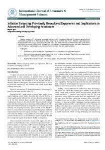
3.3 Figure 1: Linex Loss function

The Nash equilibrium:11

The central banker’s problem is to choose the sequence of instruments that minimises the present value of its loss function:

2

∞

1.8

Min Rt

1.6

Et −1 ∑ δ s L (π t + s , ut + s ) ,

(2.6)

s =0

1.4 1.2

where δ represents the discount factor. After solving for the Nash equilibrium, the inflation bias (the difference between equilibrium and targeted inflation) when an asymmetric central bank targets the natural rate of unemployment is:

1 0.8 0.6 0.4 0.2 0 -0.3

-0.25

-0.2

-0.15

-0.1

-0.05

0

0.05

D eviat io n f r o m unemp lo yment

0.1

0.15

0.2

0.25

0.3

πt = πt * +

Li nex Loss f uncti on

Figure 1 shows the plot of the central bank’s loss with respect to deviations of unemployment given a constant inflation rate when γ > 0; for more details refer to Varian (1975). When the rate of unemployment, ut , is above its natural rate or the desired rate, ut * , the exponential term in (2.5) eventually dominates and the loss increases exponentially. On the other hand if ut < ut * , it is the linear term that becomes progressively more important so loss will increase “linearly”. The converse holds when γ < 0. This is another striking feature of the loss function in (2.2). It is clear from figure 1 that the loss associated with a positive deviation from ut * is greater than a negative deviation of the same magnitude. The Linex loss function used here also incorporates the usual quadratic loss function as a special case, that is when γ = 0.

λφ ⎡ 12 γ ⎢e γ ⎣

σ t2

2

⎤ − 1⎥ ⎦

(2.7)

where σ t2 is the conditional variance of the unemployment rate or output shock and φ is the parameter from the Phillips curve, assumed to be positive. So the level of inflation bias depends on the preference parameter γ and the conditional variance of the economy’s output shocks. For the special case where preferences are quadratic, the bias could be computed by taking: ⎤ λφ ⎡ 12 γ σ − 1⎥ = 0 . ⎢e γ ⎣ ⎦ 2

lim γ →0

2 t

With quadratic preferences, the inflation bias is zero. One important observation we can make about (2.7) is that the sign of the inflation bias depends on whether γ < or > 0. According to this model there is a disinflation bias if γ < 0, where the central banker attaches a smaller loss to positive than negative deviations from the unemployment target. The converse case, where γ > 0, would be more plausible for most central banks around the world. Intuitively, this means that central bankers are more concerned about recessions than boom times. When there is a lot of uncertainty about the future state of the economy, central banks prefer

11

The details of solving for the Nash equilibrium is omitted here; see Ruge-Murcia (2001).

16

17

lower interest rates to high; this leads to a positive inflation bias. Another thing is that the level of inflation bias is monotonically increasing in γ. The inflation bias hypothesis proposed by Cukierman and Gerlach (2003) and Ruge-Murcia (2001) is based on only two assumptions: i) there is uncertainty about next period’s realisations of inflation and output and ii) central bankers have asymmetric preferences. I formally test this proposed inflation bias hypothesis for New Zealand in the next section.

4

Methodology to improve inflation targeting

4.1

Systematic patterns in inflation error

The proposed solution by Rowe (2002) to improve inflation targeting assumes that the forecasting equation (1.8) includes all the relevant indicators, with It representing the policy maker’s real time information set (a vector of indicators):

π t − π * = γ + φI t −k + ε t .

(1.8)

However, in practice, data may not be available for all indicators in the information set, and it is clearly not feasible to include all indicators in the forecasting equation.12 Rowe (2002) showed that the proposed solution is robust to missing indicators and that policy advice from even a simple linear regression is good advice. However, policy advice from the multiple regression, including all relevant indicators and allowing for interaction between them, would be even better.

4.1.1 The data

The Reserve Bank of New Zealand Act (1989) took effect from February 1990. The initial policy targets agreement under the Act required the RBNZ to maintain inflation in the range of 0-2 per cent; in 1996 this was changed to 0-3 per cent and as of mid-2002 the target band has been 1-3 per cent. For the analysis of this paper, the mid-point of the target band was taken as the operational target, π*.13 Quarterly data for the period 1989Q1 to 2002Q2 were selected for the analysis.14 Three different inflation measures were used, these being total inflation (CPI), weighted median inflation (CPIM) and inflation excluding interest & GST (CPIX). Using different inflation measures could help us to overcome the question of which inflation measure the Bank actually targets and it would also act as a robustness check on the results. The midpoint of the target band was subtracted from the inflation measures to form three new variables. These new series can be interpreted as the actual deviations of inflation from target, πt-π∗.15 A set of 27 indicators was chosen based on economic intuition.16 These indicators include domestic demand factors, cost side factors, inflation pressure indicators, money, exchange rates, foreign inflation and interest rates. For a more detailed description of the series, refer to appendix 2. Final revised data was used in all estimations. Ideally, it would have been better to use vintage data as available to the policy makers at the time of the decision making, but this was not possible. Consequently, startingpoint uncertainty is not accounted for. Nevertheless, over a sufficiently long time horizon, errors due to this source should in principle cancel each other out. The subject is left to future research looking at the effect of revised data and policy error. The 90-day interest rate was chosen as a proxy for the policy maker’s instrument. This is partly because the mechanism for implementing 13 14

15 12

This is due to strong multicollinearity among the indicators and the limited degrees of freedom available due to the limited sample size. For example, different measures of inflation over the business cycle may be highly correlated.

16

The reaction function in section 4.3 was adjusted to allow for the non-constant target. This time period selected corresponds to the time RBNZ Governor Don Brash was in office. The denotations are CPIE, CPIME and CPIXE for total inflation, median inflation and inflation ex interest & GST respectively. We started investigating 35 variables but the high correlation among some of the indicators and the limited sample size meant that some had to be dropped.

18

19

monetary policy in New Zealand has changed over the past 10 years, making the overnight and other short-term interest rates less suitable. The 90-day rate is an interest rate on which monetary policy has had an immediate and predictable impact over the entire sample period.

I chose the automated general-to-specific (Gets) approach to model selection developed recently by Hendry and Krolzig (2001) to help identify the final model. Monte Carlo studies have shown that PcGets selects models with accuracy close to what one would expect if its data generating process were known. The multi-path searches check for hidden relationships, and highlight the relevant explanatory variables, thus avoiding path dependency problems, which can seriously affect the properties of a simplified search procedure. However, the final model is quite sensitive to what variables are included in the starting full model. For a more detailed review of the simplification algorithm refer to the PcGets manual (Hendry and Krolzig, 2001) and Owen’s (2003) review of the software.

Unit root tests for all the variables are presented in appendix 3. All variables are stationary at the 10 per cent level apart from AU10Y, US90D and US10Y. See appendix 3 for a more detailed discussion of the unit root results. 4.1.2 Econometric technique – multiple regressions

To take into account the interactions between the indicators, we need to look at the multivariate relationship between the indicators and the target variable. I ran ordinary least squares (OLS) regressions with the dependent variable being the deviation of inflation from the target, and the independent variables formed by the various indicators in the policy maker’s information set lagged eight quarters. The eight quarter lag reflects the fact that it takes roughly eight quarters 17 for changes in the interest rate to have a major impact on the rate of inflation.18 I repeated this for each of the three different inflation measures. It is not obvious which indicators to include in the regression equation. Ideally, one would want to include all variables in the policy maker’s information set as potential indicators of future inflation outcomes; this would allow us to examine whether the Bank is reacting optimally to each of them. The problem arises from possible multicollinearity among the independent variables, which could cause each indicator to be statistically insignificant, even if the set of highly correlated indicators as a whole is strongly significant in explaining variation in future inflation deviations from target. With a limited sample size, normally we would turn to economic theory to see if that can shed some light on the problem of finding the “right” specification for the model. However, even if economic theory can tell us which variables are indicators of inflation, ie which indicators the Bank responds to, it does not provide any information as to whether the Bank is likely to underreact, overreact or react optimally to that indicator. 17 18

Eight quarters is the length of the policy lag within the RBNZ’s FPS model. Although policy lags vary across different variables, for optimal policy we only require the correlation between variables and inflation deviations from target to be zero after eight quarters.

4.2

Inflation bias with asymmetric loss function

According to (2.7), the amount of inflation bias depends on three things: the parameters φ from the Phillips curve, γ from the loss function and the conditional variance of output over time. The only variation on the right hand side of (2.7) comes from the conditional variance term; it would not be possible to identify the structural parameters λ, φ and γ separately. Rewriting (2.7): ⎛

πt = ⎜πt * − ⎝

λφ ⎞ λφ ⎛ 12 γ + ⎜e γ ⎟⎠ γ ⎝

σ t2

2

⎞ ⎟ + εt . ⎠

(2.7a)

An estimate of the constant term in (2.7a) will only yield a combination of φ the structural parameters, π t * − 2 . On the other hand, the time series γ

variation in σ t2 alone would not be able to identify λ, φ and γ. To overcome the identification problem I approximate the exponential term in 1

(2.7) by taking a first order Taylor Series expansion of produce: ⎡ λφ ⎛ 1 γ 2σ t2 ⎞ ⎤ λφ ⎛ 1 2 2 ⎞ λφ 1 + λφγσ t2 . f ⎢ ⎜ e2 ⎟⎥ ≈ ⎜1 + γ σ t ⎟ = 2 ⎠ γ ⎠ ⎦⎥ γ ⎝ 2 ⎣⎢ γ ⎝

e2

γ 2σ t2

about zero to

(2.7b)

20

21

Substituting (2.7b) back in (2.7a), inflation can be written in reduced form as:

ε t ~ iid (0, σ ε2 ) and E (ηt ε t ) = σ υ2 with finite higher moments. The usual way of

π t = α + βσ t2 + ε t ,

(2.8)

where α = π * and β = λφγ . Although the parameter estimate of β cannot 1 2

reveal the structural parameters λ, φ and γ, its sign is informative regarding the asymmetry in the central banker’s preferences. Since λ and φ > 0, if the parameter estimate of β is positive, that would imply γ > 0. This corresponds to the idea that the central banker places more weight on positive than negative unemployment deviations from the target. The Barro-Gordon model yields a linear relationship between inflation and current output; in contrast, this model predicts a nonlinear relationship between inflation and lagged output.19 4.2.1 The data

Data on the quarterly CPIX inflation rate and quarterly seasonally adjusted real GDP growth from 1982Q2 to 2003Q1 were used for the analysis. The chosen time frame coincides with the longest time series available for the two variables. A dummy variable taking the value of 1 from 1990Q1 to 2003Q1 (0 prior to 1990) was formed to account for the effect of the introduction of the Reserve Bank Act in 1989. 4.2.2 Econometric techniques – generated regressors

Consider a more general form of (2.8): π t = α + βσ + θ X t + ε t , 2 t

(2.8a)

σ t2 = E ( yt − yt* ) 2 ,

and

σ t2 = ηt2 + ϕt .

where X t is a vector of covariates; yt* is the anticipated value of yt . Assume that ηt = yt − yt* is available and ηt ~ iid (0, σ t2 ) ; furthermore, 19

Under an autoregressive specification for the variance of output shock, σ t2 .

obtaining parameter estimates for α, β and θ is by finding the proxy for σ t2 ,ηt2 , then regressing π t against X t and ηt2 . Pagan (1984) shows that this two-step estimation method is almost always inconsistent. The problem arise because ηt2 is only a proxy for σ t2 with error ϕt . Substituting ηt2 into (2.8a) will introduce another error term ϕt into the regression. To see this formally, rewrite equation (2.8a) as: π t = α + θ X t + βηt2 + β (σ t2 − ηt2 ) + ε t .

(2.8b)

The estimators α, β and θ are consistent only if: i)

P T −1 ∑ X t ⎡⎣ β (σ t2 − ηt2 ) + ε t ⎤⎦ ⎯⎯ →0 ,

ii)

P →0, T −1 ∑ηt2 ⎡⎣ β (σ t2 − ηt2 ) + ε t ⎤⎦ ⎯⎯

(2.9)

which implies: Tlim T −1β ∑ E (σ t2ηt2 − ηt4 ) = lim T −1β ⎡⎣ ∑ σ t4 − E (ηt4 ) ⎤⎦ . T →∞ →∞ Even though the law of large numbers for independently distributed random variables ensures that the second moments will converge, it would be unlikely that T −1 ∑ηt4 = E (ηt4 ) . Pagan (1984) also demonstrates that the inconsistency between the 2-step estimator and β could be very large. −1 4 4 T −1 ∑ E (ηt4 ) ⎛ βˆ ⎞ lim T ⎡⎣ ∑ σ t − E (ηt ) ⎤⎦ − Tlim →∞ E ⎜⎜ ⎟⎟ = T →∞ . lim T −1 ∑ E (ηt4 ) ⎝β ⎠ T →∞

(2.10)

The inconsistency is proportional to β by the above factor. In the case where ηt is normal, the inconsistency could be up to 66 per cent of the actual value of β. An alternative estimating procedure is to use Full Information Maximum Likelihood (FIML) to find the parameters α, β and θ by maximising the joint likelihood. This is often computationally intensive and it would be very hard to write down the joint likelihood for π t and ηt especially when E (ηt ε t ) ≠ 0 .

22

23

Another way to estimate β and its standard error is to use non-parametric bootstrapping methods to obtain the empirical distribution of β. First, I estimate a GARCH model for the quarterly growth in GDP. Using the estimated model, I could then generate bootstrap samples of ηˆit2 . Now, estimate the regression in (2.8a) using ηˆit2 to obtain αˆi , βˆi and θˆi . Repeat the process n times to obtain the empirical distribution of α, β and θ. For example, from the empirical distribution of β, made up of βˆ1 , βˆ2 , βˆ3 ,......., βˆn , we could compute the mean and standard deviation to approximate the parameter β and its standard error. However, even though the generated bootstrap samples contain the characteristics of the data generating process from the GARCH model, it fails to maintain the timing of the variations to match the original data.20

where υt is the deviation of output growth from trend and yt is the output growth rate. The appropriate instrument for the model would be ηt2−1 . To obtain a consistent estimate of the parameters α, β and θ, I estimate the following equation:

For this study, I have chosen to use instrumental variables (IV) estimation to overcome the parameter inconsistency problem. If ηt ~ iid (0, σ t2 ) , then ηt2−1 (σ t2 − ηt2 ) = σ t2ηt2−1 − ηt2ηt2−1 = 0 . This no longer requires the fourth moment of ηt to converge; the convergence of the second moment alone is enough to ensure that the condition in (2.9) holds. For the formal proof of this result and asymptotic properties of the IV estimator, see Theorem 10 in Pagan (1984). I use the variance of quarterly GDP growth as a proxy for the conditional variance, σ t2 . This proxy is formed by taking the fitting values from a GARCH model modeling the variance of GDP growth. A GARCH(p,q) could be represented by: p

η = αˆ 0 + ∑ αˆ υ 2 t

j =1

2 j t− j

q

+ ∑ λˆk y k =1

2 t −k

(2.11)

π t = α + θ X t + βηt2 + ε t ,

(2.8c)

with ηt2−1 as an instrument for ηt2 .

5

Results

5.1

Systematic patterns in inflation error

5.1.1 Simple correlations

I examine deviations of the three different inflation definitions from the target variable, total inflation (CPIE), median inflation (CPIME) and inflation excluding interest & GST (CPIXE). The correlations are presented in the following three tables.21 Assuming the control lag is eight quarters, deviations of inflation from target should be uncorrelated with the instrument and each indicator after 8 quarters. Correlations bigger than 0.2222 are considered to be statistically significant at the 10 per cent level; while correlations bigger than 0.2723 are considered to be significant at the 5 per cent level. The first point to note is that the number of significant correlations declines as we move from total inflation to inflation excluding interest & GST measures. It appears that the Bank is doing a better job at targeting CPIX than other inflation measures, which is not surprising given that the Policy Target Agreement (PTA) explicitly states maintaining price stability as measured by CPIX as its primary objective. Next, I look at the correlations between deviations of inflation from target and the Bank’s instrument as proxied by the 90-day bill rate. For two of 21 22

20

I have produced 10,000 bootstrap estimates for each parameter estimates. However, due to the problem explained above, those estimates do not represent the true value of the parameter of interest.

23

For a full table of the correlations, please refer to appendix 4. Computed as 1.645 / T , where T is the sample size of 54. Indicated by lightly shaded regions in the tables. Computed as 1.96 / T , where T is the sample size of 54. Indicated by darkly shaded regions in the tables.

24

25

the inflation measures, CPI and CPIM, the correlations appear to be nonsignificant after the relevant adjustment horizon. Initially, the correlations are positive then quickly decay to zero, which suggests that higher inflation leads the Bank to raise the interest rate, but it takes several quarters before inflation returns to target. The correlations for CPIXE follow the same pattern but the magnitudes of the correlations are not statistically significant at the 10 per cent level.

Table 1: Sample correlations between CPIE and various indicators Lead A90D AUDR CPIE CPIXE CR CREDIT INFRATEH NZ90D MPR TWIR UNEMPR USDR XPR

4 0.12 0.05 0.04 0.03 0.05 -0.01 0.32 0.31 -0.52 0.23 0.37 0.22 -0.59

5 -0.03 -0.07 -0.07 -0.11 -0.04 -0.16 0.24 0.27 -0.45 0.13 0.45 0.09 -0.56

6 -0.18 -0.19 -0.13 -0.23 -0.21 -0.28 0.11 0.22 -0.38 0.02 0.44 -0.03 -0.49

7 -0.26 -0.22 -0.22 -0.32 -0.28 -0.38 -0.02 0.19 -0.24 -0.09 0.42 -0.12 -0.32

8 -0.33 -0.24 -0.27 -0.32 -0.29 -0.39 -0.10 0.16 0.01 -0.23 0.37 -0.2 -0.11

9 -0.39 -0.19 -0.28 -0.26 -0.28 -0.37 -0.15 0.13 0.18 -0.27 0.31 -0.26 0.06

10 -0.39 -0.08 -0.28 -0.23 -0.27 -0.39 -0.19 0.10 0.22 -0.2 0.27 -0.3 0.16

11 -0.35 -0.05 -0.3 -0.26 -0.24 -0.4 -0.24 0.06 0.20 -0.28 0.25 -0.36 0.19

12 -0.26 -0.04 -0.33 -0.32 -0.17 -0.42 -0.28 -0.02 0.07 -0.3 0.25 -0.28 0.12

13 -0.17 -0.05 -0.37 -0.39 -0.05 -0.39 -0.29 -0.11 -0.01 -0.22 0.23 -0.21 0.04

14 -0.08 -0.11 -0.39 -0.42 0.06 -0.31 -0.26 -0.20 -0.03 -0.14 0.16 -0.05 -0.03

Table 2: Sample correlations indicators Lead A90D AUDR CPIE CPIXE CR CREDIT INFRATEH NZ90D MPR TWIR UNEMPR USDR XPR

4 0.06 -0.08 -0.24 -0.25 0.10 0.03 0.09 0.15 -0.36 0.08 0.45 0.1 -0.56

5 0.05 -0.16 -0.33 -0.4 -0.04 0.01 0.00 0.09 -0.22 -0.05 0.46 -0.1 -0.42

6 0.03 -0.29 -0.34 -0.47 -0.27 0.03 -0.11 0.05 -0.12 -0.21 0.38 -0.3 -0.25

Table 3: Sample correlations indicators Lead A90D AUDR CPIE CPIXE CR CREDIT INFRATEH NZ90D MPR TWIR UNEMPR USDR XPR

4 -0.05 0.20 -0.03 -0.05 0.12 -0.02 0.30 0.04 -0.60 0.27 0.25 0.24 -0.59

5 -0.03 0.02 -0.10 -0.14 0.10 -0.17 0.30 0.04 -0.52 0.20 0.29 0.15 -0.54

6 -0.02 -0.10 -0.10 -0.18 -0.03 -0.30 0.26 0.08 -0.41 0.12 0.24 0.06 -0.45

between 7 0.02 -0.37 -0.36 -0.45 -0.32 -0.03 -0.22 0.05 0.03 -0.32 0.28 -0.35 -0.01

CPIME

8 -0.01 -0.38 -0.3 -0.33 -0.28 -0.08 -0.29 0.04 0.3 -0.42 0.17 -0.35 0.22

9 -0.04 -0.27 -0.21 -0.16 -0.24 -0.12 -0.33 0.00 0.44 -0.33 0.09 -0.3 0.35

between 7 0.02 -0.15 -0.11 -0.20 -0.07 -0.39 0.17 0.12 -0.28 0.03 0.21 0.02 -0.28

8 0.04 -0.16 -0.13 -0.20 -0.06 -0.39 0.09 0.15 -0.06 -0.14 0.16 -0.09 -0.10

10 -0.07 -0.10 -0.16 -0.06 -0.2 -0.18 -0.32 -0.05 0.44 -0.15 0.07 -0.28 0.4

CPIXE

9 0.04 -0.07 -0.10 -0.14 -0.05 -0.36 0.03 0.15 0.08 -0.12 0.13 -0.11 0.00

10 0.03 0.04 -0.12 -0.15 -0.04 -0.41 0.00 0.12 0.08 -0.04 0.13 -0.12 0.04

and

11 -0.09 0.01 -0.19 -0.07 -0.14 -0.22 -0.29 -0.09 0.32 -0.09 0.08 -0.21 0.35

12 -0.13 0.05 -0.25 -0.15 -0.06 -0.22 -0.25 -0.15 0.09 -0.13 0.1 -0.13 0.21

and 11 0.01 0.07 -0.17 -0.20 -0.04 -0.40 -0.05 0.10 0.06 -0.12 0.14 -0.21 0.04

12 -0.02 0.01 -0.22 -0.27 -0.01 -0.41 -0.08 0.04 -0.04 -0.19 0.17 -0.19 -0.04

various 13 -0.15 0.05 -0.29 -0.24 0.04 -0.23 -0.2 -0.2 -0.07 -0.06 0.09 -0.07 0.06

14 -0.16 -0.01 -0.31 -0.31 0.12 -0.22 -0.17 -0.25 -0.12 -0.04 0.04 0.03 -0.06

various 13 -0.04 -0.09 -0.29 -0.36 0.04 -0.42 -0.11 -0.02 -0.07 -0.20 0.18 -0.21 -0.07

14 -0.05 -0.21 -0.31 -0.37 0.13 -0.33 -0.11 -0.08 -0.04 -0.17 0.15 -0.11 -0.09

In more detail, the medium inflation measure’s correlations turn negative after 9 quarters. On the other hand, the correlation for both total inflation and inflation without interest & GST turn negative after 13 quarters. This may suggest the control lag of monetary policy could be longer than 8 quarters. Erring on the side of caution, I assume that the control lag is indeed eight quarters, so that all correlations should be zero at a lag of

26

27

eight or more quarters, if monetary policy is responding optimally to the indicators. If the observed correlation between the Bank’s instrument and deviations from target is positive at lags longer than the control lag, then the Bank is not responding aggressively enough to bring inflation back to the target; likewise for a negative correlation, the Bank would have been too aggressive. At lags longer than the control lag (8 quarters), the correlations between the Bank’s instrument and deviations from target are not significantly different from zero. This means that on average the Bank has been responding optimally to inflation.

independent variables (ie equation (1.8)), was estimated by Ordinary Least Squares (OLS) using the general-to-specific (Gets) approach to model selection in PcGets (Hendry and Krolzig, 2001). Default settings in PcGets (liberal and conservative) have the significance level for variable reduction set at 0.05 and 0.1 respectively. This cut off value is too low for the purpose of this project. 24 Remember, if a variable is found to be insignificant, this does not necessary imply the variable is irrelevant; it simply means policy makers are already responding optimally to that indicator. However, significant variables would suggest policy makers had either overreacted or underreacted depending on the sign of the coefficient in the estimated equation.

Responding optimally to inflation on average does not mean the Bank was responding optimally to each indicator of inflation. It could have been overreacting to some indicators and underreacting to others, causing inflation, the exchange rate and output to fluctuate more than if it were reacting to each optimally. Ideally, it would be useful to have a look at correlations for the period after 1993 when the Bank has been through the disinflation period and is more “comfortable” with inflation targeting. If the correlations got smaller, that means the systematic mistakes mentioned above could have been due to the “learning” period of inflation targeting; and the Bank’s inflation targeting performance had improved over time. However, with less than nine years of data, we should be careful not to read too much into cross correlations that are lagged by up to 14 quarters.

The Gets model selection procedure has been criticised for amounting to data mining. The idea behind this criticism is that theory should dictate which variables are included or excluded from an estimated regression equation; otherwise it may give spurious results. However, the Gets approach is well suited for this project. Underlying economic theory may tell us which indicators are important in forecasting inflation, but it cannot determine which indicators policy makers are responding to in a suboptimal way. There is no prior information to address this problem; the best we can do is to assume that policy makers are on average responding optimally to the indicators, i.e. that there is an equal probability that the Bank will under or over-react to any one indicator. Furthermore, Rowe (2002) has shown that policy advice based on a smaller set of indicators is still valid and the result is robust to missing indicators.

5.1.2 Multivariate regressions

Policy recommendations discussed in the previous section should be treated with great caution. Each of the suggestions from the simple correlation analysis should be taken as independent advice only; it cannot be used jointly in the policy making process. However, it does provide motivation for more in-depth research in the area, given the possibility that the Bank may have made systematic mistakes in policy setting over the inflation targeting period. We proceed to look at the multivariate relationships between the indicators and deviations of inflation from target. This allows the indicators to interact with each other, allowing joint policy recommendations in the decision making process.

In Section 4.1, I reported evidence suggesting that the Bank has paid the most attention to inflation excluding interest & GST (CPIX), so I will mainly concentrate on this inflation measure in this section. 25 Table 4 shows the final estimated regression from the Gets algorithm with deviations of CPIX from target as the dependent variable and the various indicators lagged 8 quarters26 as the independent variables. I also ran the model selection process with capacity utilisation (as a proxy for the output gap) forced into the model to control for the business cycle. 24

25

The “forecasting” equation, with deviations of inflation from target as the dependent variable and the various indicators (lagged eight quarters) as

26

For this project, I have used a 50 per cent significance level as the cut off point for deletion of variables in both the pre-search and multiple path searches. Although not presented here the results for the other two inflation measures are included in appendix 5. From looking at the simple correlations analysis most of the significant correlations turn to zero after eight lags; this provides further evidence that the Bank’s adjustment horizon is indeed eight quarters.

28

29

Table 4: Final estimated forecasting equation Coeff

StdError

t-value

Constant

Indicators

3.03

0.72

4.22

P-Value 0.00*

A90D(-8)

-0.18

0.08

-2.16

0.04*

AUDR(-8)

-0.09

0.03

-2.87

0.01*

AUINFRATE(-8)

0.10

0.08

1.25

0.22

CR(-8)

0.20

0.11

1.77

0.09

CREDIT(-8)

-0.15

0.06

-2.55

0.02*

INFRATEH(-8)

-0.10

0.05

-1.95

0.06

MIGR(-8)

-0.05

0.02

-2.40

0.02*

OILPRI(-8)

-3.37

1.63

-2.07

0.05*

UNEMPR(-8)

-0.02

0.01

-1.76

0.09

USDR(-8)

0.04

0.01

2.60

0.01*

R2

0.6654

Adjusted R2

0.5697

RSS Sigma Loglikelihood

23.536 0.82 15.412

AIC

-0.19181

N

46

P

11

Model Diagnostics: TESTS:

Value

Chow(1996:4)

1.117

Prob 0.43

Chow(2001:2)

0.5685

0.6874

Normality test

0.1396

0.9326

AR 1-4 test

2.5664

0.0891

ARCH 1-4 test

0.5664

0.6891

Hetero test

2.221

0.2781

correlated with the Australian short term interest rate and PcGets failed to distinguish the effects from the two. Both the Australian interest rate and expected inflation had negative signs, but we can not distinguish which one (or both) the Bank had overreacted to. Here I have decided to report results for the model that includes the Australian interest rate.28 Despite this, the resultant estimates of other variables in the final model do not change much across the two different starting specifications. The R2 of the selected final model was 0.6654, ie 66.54 per cent of the variation in inflation deviation from target was explained by the estimated regression. This suggests that there is scope for improvement in achieving targeted inflation. If policy makers were behaving completely optimally, we would expect the R2 to be near zero; this would have implied that the indicators we looked at had no further “value” in forecasting inflation deviations and any observed inflation deviations from target were just random errors. Even though the forecasting equation tells us whether or not the Bank has been responding optimally in the past, it fails to address the question, “What should policy makers do in order to improve inflation targeting?” To address this we need to know what the policy maker has been doing in the past and, in particular, what their response was. We start by estimating the Bank’s actual reaction function, together with the information from the forecasting equation that tells us which direction the actual reaction function ought to be adjusted. This will give us some idea of what the optimal reaction function might look like. Recall that the partial derivative of Rt with respect to It is: ∂Rt δ =− β ∂I t

* Significant at the 5 per cent level.

The general unrestricted model (Gum) included 27 indicators,27 these were later reduced to 10 using the Gets algorithm. I have also considered other specifications for the starting model as a robustness check for the final model considered before. It appears inflation expectations are highly 27

One of the shortfalls with PcGets is that it failed to distinguish the effect from highly correlated (correlation above 0.9) explanatory variables. Some of these highly correlated variables had to be taken out manually, such as different measures of inflation expectations. At the end, 27 variables were left in the general model unrestricted model.

,

so

∂Rt δ 0⇔δ 0⇔ 0. β ∂I t

For example, if an indicator were found to have a positive coefficient in the forecasting equation and a positive coefficient in the reaction function, we can say that the Bank has been underreacting to the indicator by 28

The NZ and AU short term interest rate had a correlation of 0.9.

30 reacting positively. In this case,

δ% δˆ δ% < ; the revised estimate of the ratio % ˆ β% β β

δˆ

more negative than ˆ , therefore the Bank should adjust its response β upwards. Intuitively, the Bank has increased interest rates by too little following an increase in the indicator (since the indicator is positively related to interest rates in the reaction function). The advice here is to increase interest rates by even more following an increase in the indicator. For a more detailed explanation on how to interpret the coefficient estimates, refer to appendix 1. The most difficult task so far is estimating the Bank’s reaction function. The reaction function is used to capture the Bank’s behaviour over the sample period. For simplicity, I have assumed the Bank’s reaction function over this period to be linear; the estimated reaction will only represent the average response of the Bank over the period. Table 5 shows the estimated reaction function, equivalent to (1.2b), using the 90-day interest rate as a proxy for the instrument.29

31

Table 5: Actual reaction function Coeff

StdError

t-value

Constant

Indicators

2.44

0.77

3.16

P-Value 0.00*

A90D(-1)

0.6

0.1

5.84

0.00*

AUDR(-1)

-0.04

0.04

-1.18

0.25

AUINFRATE(-1)

0.02

0.05

0.35

0.73

CR(-1)

-0.17

0.13

-1.31

0.2

CREDIT(-1)

0.03

0.07

0.35

0.73

INFRATEH(-1)

0.27

0.06

4.72

0.00*

MIGR(-1)

0.01

0.01

0.72

0.48

OILPRI(-1)

-1.15

1.31

-0.88

0.38

UNEMPR(-1)

0.01

0.01

0.73

0.47

USDR(-1)

-0.03

0.01

-2.75

0.01*

CPIE(-1)

0.14

0.15

0.97

0.34

R2

0.8578

Adjusted R2

0.8118

RSS

26.472

Sigma

0.8035

Loglikelihood

18.396

AIC

-0.24138

N

53

P

12

Model Diagnostics: Value

Prob

Chow(1996:4)

1.4236

0.2401

Chow(2001:2)

0.6135

0.6902

Normality test

5.596

0.0609

AR 1-4 test

2.5405

0.0603

ARCH 1-4 Test

0.812

0.5275

Hetero test

0.772

0.7209

* Significant at the 5 per cent level.

29

A second reaction function was estimated using PcGets with all the indicators in the starting model (shown in appendix 4). However, this is not that helpful in terms of interpreting the results from the forecasting equation, since it does not include some of the indicators that appears in the forecasting equation but it serves as a good robustness check for the first reaction function. Generally the signs of coefficients are the “right” ones and it seemed to agree with the results from the first reaction function.

I have used the same set of indicators in the forecasting equation as independent variables in the reaction function. Deviations of inflation from target lagged one quarter were added to the reaction function to adjust for the non-constant inflation target. For a given set of values in the information set we would expect the Bank to set the instrument differently

32 if inflation were 2 per cent from target as opposed to 1 per cent. The aim here is not to estimate the “state of the art” reaction function for future policy making but rather to see to which indicators the Bank is responding and to which indicators it is not. Together with the signs of the coefficients, it will help us to interpret the forecasting equation in a more meaningful way.

33

Figure 3: Reaction function

Surprisingly, the estimated reaction function explained over 85 per cent of the variations in the 90-day interest rate. However on the negative side, some of the variables appear to be insignificant, whereas normally we would expect them to have a significant effect on policy maker’s decisions. This could be due to the oversimplified linear specification of the reaction function, and also because the Bank uses current as well as past information in setting policy whereas my analysis only includes past information.30 5.1.3 Summarising the results

Figures 2 and 3 show the actual versus fitted values and residual plot for both the forecasting and reaction functions. The estimated forecasting equation does show similar patterns with actual deviations of inflation from target.

Figure 2: Forecasting equation

The coefficient on the short-term Australian interest rate31 is negative and it is statistically significant in the forecasting equation; the reaction function shows strong positive response to this indicator by the Bank. This suggests that the Bank was overreacting to this indicator. The domestic interest rate was increased by too much when the Australian monetary authority lifted Australian interest rates. Taken together, the results suggest the Bank should increase (decrease) the domestic interest rates by less than what it had when it sees an increase (decrease) in Australia interest rates. Evidence to support this could be found in 1993 where the Australian interest rate was quite low, and the Bank responded by lowering the domestic interest rate. However, this overreaction to the Australian interest rate contributed to inflation rising above target in 1995. The change in the AU/NZ exchange rate has a significant negative coefficient in the forecasting equation. The coefficient on the variable is negative but not statistically significant in the reaction function. It is nevertheless plausibly signed according to economic theory, that is an appreciation of the exchange rate will lead the Bank to decrease interest rates. This is because an appreciation of the New Zealand dollar is normally seen to have a negative impact on short- to medium-term inflation. So here, it is considered to be economically significant. This 31

30

To minimise the simultaneity bias.

This could be viewed as a proxy for world interest rate movements. The Australian short-term interest rate shares similar trends with US short- and long-term interest movements (excluded here due to the multicollinearity problem).

34

35

means the Bank had been underreacting to changes in the Australian/New Zealand dollar exchange rate. Putting it together, the Bank should have reduced the 90-day interest rate by even more in response to an appreciation of the New Zealand dollar against the Australian dollar.

in response to an increase in oil prices, accommodating the initial impact of the oil price shock. Together, it indicates that the Bank had underreacted to the increase in oil prices. The somewhat surprising advice here is to accommodate oil price shocks by even more. This result could be due to the fact that the coefficient estimate from the reaction function was not significant, whereas I have treated it as negative.

For the US/NZ exchange rate, its coefficient in the forecasting equation is positive and significant; the sign of the coefficient in the reaction function is negative and significant. The Bank has therefore been overreacting to changes in the US/NZ exchange rate. On average, policy response had been negative over the sample period, ie, an appreciation of the New Zealand dollar against the US dollar led the Bank to decrease the interest rate. Taken together, it suggests the Bank should have decreased the interest rate by less than they did following an appreciation of the NZ dollar against the US. This is not at all surprising considering the value of New Zealand’s exports denominated in US currency has increased significantly over this period; an appreciation of the NZ dollar against the US would have a significant impact on the overall level of economic activity and would therefore lower the rate of inflation. The Trade Weighted Index (TWI) did not get selected into the final model, which means the Bank had responded optimally to changes in the value of the NZ dollar but it needs to focus more on individual cross exchange rates. During the sample period, the Bank underreacted to the Australian dollar and overreacted to the US dollar, on average. The coefficient for credit growth is negative and significant in the forecasting equation. The reaction function carries a positive sign but the coefficient is not significant. As we might expect, the Bank tends to respond to higher credit growth by putting up the interest rate. In this case, the evidence suggests that the Bank has been overreacting to credit growth. In other words, the Bank should have increased interest rates by less when credit growth increased. Changes in net migration also carry a negative sign in the forecasting equation, and a positive coefficient in the reaction function. The Bank tended to overreact by increasing the interest rate by too much when net migration increased. Again the advice here is to adjust the response downwards to changes in net migration. Another interesting result is the negative and significant coefficient for changes in the oil price. The coefficient from the reaction function was negative. This tends to suggest the Bank had been lowering interest rates

No other indicators are statistically significant in the forecasting equation, which suggests that either the Bank was responding optimally to these indicators, or the method used here is not powerful enough to suggest otherwise. The results discussed here are the Bank’s average responses over the sample period. For policy advice to be valid the Bank’s reaction function must be the same over the sample period. In the next section, I look at the recursive statistics for the estimated coefficients to see if those shed light on the issue of consistency in the Bank’s monetary policy settings. 5.1.4 Recursive statistics

Recursive statistics on the estimated coefficients in the forecasting equation are calculated by first estimating the regression coefficients using the smallest sample size possible. Then these regression coefficients are re-estimated by adding one more observation at a time. In figure 3, the solid lines show the estimated coefficients over time and the dotted lines indicate the 95 per cent confidence intervals. Overall, most of the parameters remained constant over time. For the Australian short-term interest rate, the coefficient was positive and significant at the start of the sample period, but over time, the coefficient moved below zero. For changes in net migration, the estimated coefficient changed over the sample period from significantly positive to significantly negative. Another interesting result is the change in US/NZ exchange rate. The coefficient was near zero at the beginning of the period, but increased sharply in 1998 and remained significantly positive thereafter. Looking at other variables in the forecasting equation, the relationship between these indicators and inflation deviation from target remained constant over time. It appears there was no major change in the Bank’s behaviour over the sample period with respect to those indicators 32 32

Other than the three mentioned above.

36

37

5.2 Figure 4: Recursive statistics for parameters in the forecasting equation 4.0

.1

.15

3.5

.0

.10

-.1

.05

3.0 2.5

-.2

.00

-.3

-.05

2.0 1.5 1.0

-.4

-.10

0.5

-.5

-.15

1987 1988 1989 1990 1991 1992 1993 Recursive C(1) Estimates

1987 1988 1989 1990 1991 1992 1993

?2 S.E.

Recursive C(2) Estimates

Recursive C(3) Estimates

.3

.2

.15

.2

.1

.1

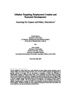
5.2.1 Estimated GARCH model

To model the conditional variance in the quarterly GDP growth, σ t2 , a series of GARCH models (equation (2.11)) was fitted to the data. The GARCH (1,1) model provided the best fit according to the AIC selection criteria shown in table 6. This was taken to be the preferred model for the conditional variance of quarterly GDP growth. Table 7 presents the maximum likelihood estimates from the GARCH(1,1) model and its asymptotic standard errors.

1987 1988 1989 1990 1991 1992 1993

?2 S.E.

.20

.10

Inflation bias

?2 S.E.

Table 6: AIC for GARCH models.

.0

.0 .05

-.1

Models

-.1 .00

-.2

-.2

-.05

-.3

-.3

-.10

-.4 1987 1988 1989 1990 1991 1992 1993 Recursive C(4) Estimates

?2 S.E.

.5

-.4 1987 1988 1989 1990 1991 1992 1993 Recursive C(5) Estimates

1987 1988 1989 1990 1991 1992 1993

?2 S.E.

Recursive C(6) Estimates

.12

8

.08

4

?2 S.E.

.4 .3 .2 .1

.04

0

.00

-4

-.04

-8

GARCH (0,1) GARCH (1,0) GARCH (1,1) GARCH (2,1) GARCH (1,2) GARCH (2,2)

No of parameters 1 1 2 3 3 4

Neg Likelihood 90.566 96.881 89.406 92.332 90.981 90.694

AIC

183.132 195.762 182.812 190.664 187.962 189.388

.0 -.1 -.2

-.08 1987 1988 1989 1990 1991 1992 1993 Recursive C(7) Estimates

-12 1987 1988 1989 1990 1991 1992 1993

?2 S.E.

Recursive C(8) Estimates

.08

.05

.06

.04

?2 S.E.

.03

.04

.02 .02 .01 .00

.00

-.02

-.01

-.04

-.02 1987 1988 1989 1990 1991 1992 1993 Recursive C(10) Estimates

?2 S.E.

1987 1988 1989 1990 1991 1992 1993 Recursive C(11) Estimates

1987 1988 1989 1990 1991 1992 1993

?2 S.E.

Recursive C(9) Estimates

C1 C2 C3 C4 C5 C6 C7 C8 C9

?2 S.E.

Constant A90D_8 AUDR_8 AUINFRATE_8 CR_8 CREDIT_8 INFRATEH_8 MIGR_8 OILPRI_8

Table 7: Maximum likelihood estimates for GARCH (1,1). Coefficient estimates α0 α1 λ1

Estimates 1.6663 0.4782 0.1315

Asy. std error 0.4033 0.1848 0.1141

t value p-value 4.132 0.00036 2.588 0.00965 1.153 0.24902

38

Figure 5: Fitted values from the estimated GARCH (1,1).

39

Table 8: Parameters Estimates for the two-step regression and IV estimation IV estimation using ηt-12 as instrument

Two-Step regression

Figure 5 shows the predicted values from the estimated GARCH (1,1) model. The conditional variances tend to mean revert back to zero quickly after a shock to the economy. Also, the conditional variances are much larger for the first half of the sample than the second half. 5.2.2 Two-step and IV estimation

Two estimation methods were used to obtain parameter estimates for α, β and θ in equation (2.8c). One is the straightforward two-step regression often used in the literature. From the analysis in Section 4.2.2, we know this will produce inconsistent coefficient estimates together with underestimated standard errors.33 A better way of performing the analysis would be to estimate the model (2.8c) via instrumental variables (IV) using lagged values of ηt2 , ηt2−1 , as an instrument for the σ t2 ’s. The parameter estimates from both methods are reported below:

33

This was simply done for comparison with the IV model.

Parameters

Coeff

Std error

t-value

p-value

Parameters

Coeff

Std error

t-value

p-value

α

2.713

0.468

5.803

0.000

α

0.933

1.249

0.747

0.457

θ

-2.847

0.293

-9.727

θ

-2.503

0.393

-6.366

0.000

β

0.647

0.189

3.424

0.000 0.001

β

1.471

0.566

2.599

0.011

Diagnostic tests:

Value

P-value

Diagnostic tests:

Value

P-value

Normality test

2.626

0.269

Normality test

0.246

0.911

AR 1- 4 test

3.039

0.006

AR 1- 4 test

3.663

0.010

ARCH 1 - 4 test

0.453

0.770

ARCH 1 - 4 test

1.102

0.405

Hetero test

3.770

0.008

Hetero test

2.353

0.063

R^2

0.6719

R^2

0.5863

The estimated model using Instrumental Variables (IV) has an R-square of 0.5863; over 58 per cent of the variation in the rate of inflation is explained by the model with the dummy variable D and the conditional variance of output growth. Apart from the autocorrelation test, most of the diagnostic tests do not show evidence of inadequate fit. The null hypothesis of no autocorrelation was rejected at the 5 per cent level, indicating there is evidence of autocorrelation present in the residuals. This is not surprising due to the lack of explanatory variables included in the regression to control for other factors that could have a significant effect on inflation. It would be interesting to investigate this inflation bias hypothesis based on a larger model for inflation, but this is left for future research. Bearing in mind the presence of autocorrelation in the residuals, I next proceed to analyse the parameter estimates. The constant from the IV regression is 0.93 but it is not statistically different from zero. The constant in this regression could be treated as the inflation target; even though the Reserve bank did not explicitly target any specific rate of inflation during the first half of sample, this could be interpreted as the implicit target given the effect of the Reserve Bank Act and the conditional variance of output growth. The estimated value of θ is -2.50 with a t-value of -6.36. Given the conditional variance of output growth, it thus appears that average inflation in New Zealand decreased by 2.5 per cent following the introduction of the Reserve Bank Act in 1989. This suggests that the

40 Reserve Bank Act may have had a significant effect on the Bank’s credibility; if so, then as the result of the institutional changes, the average rate inflation is now permanently lower. In both the two-step and IV regression, the parameter estimate for β is positive and the null hypothesis of β = 0 can be rejected at the 0.1 per cent level for the two-step regression and at the 1 per cent level for the IV regression. For the two-step regression, the estimate for β is 0.65 compared with the IV estimate of 1.47; the parameter estimate for β and its asymptotic standard error is smaller when using the two-step regression compared with IV estimation. The observed results are consistent with Theorem 10 in Pagan (1984), which shows that the two-step estimation procedure underestimates the parameter coefficients and their standard 1 errors. Recall that β = λφγ , so that the value of βˆ is uninformative about 2

the magnitude of the parameter that measures the asymmetry in the central banker’s preferences, γ. However, since λ, φ >0 by assumption of the model, a positive β automatically implies γ > 0. Thus, there is evidence to support Cukierman and Gerlach (2003) and Ruge-Murcia’s (2001) inflation bias hypothesis; as these authors found for the US and Canada, my results suggest that in the Reserve Bank’s loss function, positive deviations from potential output are weighted more heavily than negative deviations. Results from this analysis do not support the view that the Reserve Bank of New Zealand had been “too tough” on inflation. According to the estimated sign of γ, the Reserve Bank tends to react more strongly to potential economic downturns (by lowering interest rates) than to economic booms (by raising interest rates).34 Finally, I conclude that even if the Reserve Bank’s output target corresponds to the potential level of output of the economy, there are still gains, in terms of maintaining a low level of inflation, from enhancing its credibility. Recall that the level of inflation bias is monotonically increasing in γ; a reduction in the degree of asymmetry of preferences will lead to lower inflation bias.

34

This contradicts the results of Karagedikli and Lees (2004), who cannot reject that the RBNZ’s preferences regarding deviations of output from trend have quadratic during the inflation targeting period as a whole.

41

6

Conclusion

Using two new methods, I have investigated the deviations from target of New Zealand’s rate of inflation. First, Rowe’s (2002) approach examines correlations between inflation deviations from target and inflation indicators in the policymaker’s information set eight quarters earlier. In a simple framework where there is a point target for inflation, and inflation control is the sole objective of the central bank, zero correlations mean policy makers have been reacting optimally on average. By contrast, any significant correlations, whether positive or negative, in a simple or multivariate framework, would constitute evidence against optimal policy setting. Second, I examine Cukierman and Gerlach’s (2003) and Ruge-Murcia’s (2001) inflation bias hypothesis. In contrast with Kydland and Prescott’s (1977) and Barro and Gordon’s (1983) time inconsistency explanation of inflation bias, Ruge-Murcia, Cukierman and Gerlach take the view that even if a central bank targets the natural rate of unemployment or the potential level of output, some inflation bias could still exist if the loss function is asymmetric. Using Rowe’s approach and data from 1989 to 2002, I present evidence that the Reserve Bank of New Zealand has on average responded to inflation optimally. But responding optimally on average does not necessarily mean that the Bank was responding optimally to each indicator of inflation and used all available information efficiently. In particular, over the time period analysed, the Bank have systematically underreacted to increases (decreases) in the AU/NZ exchange rate and oil prices. Conversely, the Bank had overreacted to increases (decreases) in the Australian short term interest rate, US/NZ exchange rate, credit growth and changes in net migration. By responding optimally to each of the indicators, fluctuations might have been reduced in the rate of inflation, the exchange rate and output growth. It is important to keep in mind some caveats to this analysis. In particular, recommended policy changes refer only to how policy should be changed from what it was on average over the past 12 years. If the Bank’s policysetting behaviour changed significantly over that time, the data sample used in this paper cannot tell whether or not the present reaction function is optimal. Another important thing to note is that the method can only be

42

43

used to address systematic bias in observed inflation, rather than the level of average inflation bias itself.

References:

To address the issues of the average level of inflation bias, I tested the asymmetric preference inflation bias hypothesis for New Zealand using data from 1981 to 2003. I find evidence to support the inflation bias hypothesis, implying that the Bank’s loss function has been asymmetric; in particular, positive deviations from potential output seem to have been weighted more heavily than negative ones. Reducing the degree of asymmetry of preferences would in principle result in lower inflation bias.

Barro, R and D Gordon, (1983), “A positive theory of monetary policy in a natural rate model,” Journal of Political Economy, Vol 91, 589-610.

The analysis of systematic patterns in inflation helps us to draw lessons for future policy setting by highlighting items that policymakers may have overlooked in the past. One of the drawbacks of this particular analysis is that policy recommendations are qualitative rather than quantitative. Rowe’s approach can determine whether the Bank should respond more or less strongly to various indicators; however, his method does not allow one to calculate what the optimal interest rate should be to ensure that inflation will hit the target after the control lag. Further work should be pursued on improving the efficiency of the Bank’s use of selected indicators in setting policy. For the inflation bias analysis, the results obtained are based on a very simple strategic interaction of the public and the central banker; a more general equilibrium concept might produce different empirical results. Even though I have allowed for the direct effect of the institutional change in 1989, I have not accounted for other indirect effects it has probably had on inflation. Another limitation of this analysis is that the proposed model does not allow for changes in the preference parameters over time; in practice, preference parameters might plausibly change as a new governor takes office.

Blinder, A S (1998), “Central banking in theory and practice,” The MIT Press: Cambridge, MA. Cukierman, A (1999), “The inflation bias revisited,” Tel-Aviv University, Working Paper, No 38-1999. Cukierman A and A V Muscatelli (2002), “Do central banks have precautionary demands for expansions and for price stability? – Theory and evidence,” University of Glasgow, Department of Economics, Working Paper, No 2002-4. Cukierman, A and S Gerlach (2003), “The inflation bias revisited: Theory and some international evidence,” The Manchester School, Vol 71, Issue 5, 541-565. Gerlach, S (2000), “Asymmetric policy reactions and inflation,” Bank for International Settlements, Working Paper. Hendry, D F and H M Krolzig (2001), Automatic Econometric Model Selection Using PcGets, Timberlake Consultants Ltd, London. Kareken, J and R M Solow (1963), “Lags in monetary policy,” In: Stabilisation Policies: A series of research studies prepared for the Commission on Money and Credit, Englewood Cliffs, N J: PrenticeHall. King, M (1996), “How should central banks reduce inflation: Conceptual issues,” Achieving Price Stability, Federal Reserve Bank of Kansas City. Karagedikli, Ö and K Lees (2004), “Do inflation targeting central banks behave asymmetrically? Evidence from Australia and New Zealand,” Reserve Bank of New Zealand Discussion Paper DP2004/02.

44

45

Kydland, F and E Prescott (1977), “Rules rather than discretion: The inconsistency of optimal plans,” Journal of Political Economy, Vol 85, 473-490.

Svensson, L E O (1997a forthcoming), “Inflation forecast targeting: implementing and monitoring inflation targets”, European Economic Review, Vol 41, 1111-1146.

McCallum, B T (1995), “Two fallacies concerning central bank independence,” American Economic Review Papers and Proceedings, Vol 85, 201-211.

Svensson, L E O (1997b), “Inflation targeting in an open economy: strict or flexible inflation targeting?,” Reserve Bank of New Zealand, Discussion Paper, 1997/08.

McCaw, S and S Ranchhod (2002), “The Reserve Bank’s recent forecasting performance,” Reserve Bank of New Zealand Bulletin, 65, No 4, 3-23.

Varian, H (1975), “A Bayesian approach to real estate assessment”, Studies in Bayesian Economics in Honor of L. J. Savage, edited by S. E. Reinberg and A. Zellner, North-Holland: Amsterdam.

Mylonas, P and S Schich (1999), “The use of financial market indicators by monetary authorities,” OECD Economics Department, Working Papers, No 223.

Worswick, G D N (1969), “Fiscal policy and stabilisation in Britain”, Journal of Money, Credit and Banking, Vol 1, Issues 3, 474-495.

Owen, P D (2003), “General-to-specific modelling using PcGets,” Journal of Economic Surveys, Vol 17, No 4, 609-628. Pagan, A (1984), “Econometric issues in the analysis of regressions with generated regressors,” International Economic Review, Vol 25, No 1, 221-247. Peston, M H (1972), “The correlation between targets and instruments,” Economica, Vol 29, 427-431. Razzak, W A (2001), “Money in the era of inflation targeting,” Reserve Bank of New Zealand Discussion Paper, DP2001/02. Romer, D (2001), Advanced Macroeconomics 2nd Edition, Boston: McGraw-Hill. Rowe, N (2002), “How to improve inflation targeting at the Bank of Canada,” Bank of Canada, Working Paper, 2002-23. Ruge-Murcia, F J (2001), “The inflation bias when the central targets the natural rate of unemployment”, Universite de Montreal, Department de Sciences Economiques, Working paper, No 22-2001.

46

47

Appendix 1:

Appendix 2: Data descriptions

Interpreting the coefficient estimates:

Reaction function: (Economically significant)

+ve Forecasting equation:

∂Rt δ >0⇔ β% βˆ

+ve ∂Rt δ >0⇔