Implementation of new methods of speckle noise reduction in SAR images L. Bouchemakh*, Y. Smara*, M. Benali & Z. Ben Cheikh *Image Processing Laboratory, Faculty of Electronics and Computer science, Houari Boumediene University of Sciences and Technology (USTHB), B.P. 32, El Alia, Bab Ezzouar, 16111 Algiers Algeria
[email protected],
[email protected]
Keywords: speckle filtering, SAR images, wavelets transformation, MMCV filter, EMD decomposition ABSTRACT: This paper presents three methods for reducing speckle noise in SAR images. The first one, proposed by North (North & Wu 2001), is based on filtering by Minimum Coefficient of Variation (MCV) based on mathematical morphology. This method use a non-linear filter that uses local measurements of the noise in the image to guide a low pass filtering operation to act only over regions where the original signal is estimated to be homogeneous. Speckle is therefore reduced in these areas but the edges between them remain intact. The second one, proposed by Chunming (Chunming & al 2002), consists on empirical modal decomposition (EMD). It is a recent introduced tool for decomposing data into so-called Intrinsic Mode Functions (IMF). This method decomposes an image in four recursive images (vertical, horizontal, right diagonal et left diagonal) and do in the same time an appropriate smoothing by the EMD method. The reconstruction of the image is done by detecting the edge direction. The last one, proposed by Duskunovic (Duskunovic & al 2000) is based on the Daubechies wavelets decomposition with denoising detail images. This method is based on the analysis of the detail images, obtained from the wavelet decomposition of the original image. The goal of the analysis is to determine the position of real edges in the image so that false edges and noise can be removed. Comparison of these three filtering techniques with existing methods show us that they were a good compromise between reducing speckle noise, texture conservation, and edge preserving. We have done a comparative study based on statistical criteria (mean, Standard-Deviation, Speckle Index) and Visual aspect. The results obtained by these three methods tested on SAR images of Algiers city, show that we have a good reduction of speckle noise with preserving edges. 1
INTRODUCTION
Synthetic aperture radar (SAR) images are becoming more widely used in remote sensing applications. SAR uses microwave radiation to illuminate the earth’s surface, and therefore overcomes some problems associated with conventional visual remote sensing imagery. For example, SAR is not affected by cloud cover variation. The coherent microwave illumination, however, generates a multiplicative speckle noise that corrupts SAR images. We have used the properties of this speckle noise to implement two methods by IDL language (Interactive Data Language) to reduce the noise without blurring edge or other features. Many filtering algorithms have been developed to reduce speckle on SAR imagery. Nevertheless, speckle suppression and detail preservation remain the two key issues in speckle filtering. Most commonly used speckle filters have good speckle-smoothing capabilities. However, the resulting images are subject to degradation of spatial and radiometric resolution, which can result in the loss
53
of image information. For applications in which fine details and high resolution are required, the detail-preserving performance of a speckle filter should be emphasised, and may be equally important as the effectiveness of speckle reduction. This paper presents a comparative study between standard filters as Lee, Frost and Kuan filters and three other methods for reducing speckle noise in SAR images. The first one, proposed by North (North & Wu 2001), is based on filtering by Minimum Coefficient of Variation (MCV) based on mathematical morphology. This method use a non-linear filter that uses local measurements of the noise in the image to guide a low pass filtering operation to act only over regions where the original signal is estimated to be homogeneous. Speckle is therefore reduced in these areas but the edges between them remain intact. The second one, proposed by Chunming (Chunming & al 2002), consists on empirical modal decomposition (EMD). It is a recent introduced tool for decomposing data into so-called Intrinsic Mode Functions (IMF). This method decomposes an image in four recursive images (vertical, horizontal, right diagonal et left diagonal) and do in the same time an appropriate smoothing by the EMD method. The reconstruction of the image is done by detecting the edge direction. The last one, proposed by Duskunovic (Duskunovic & al 2000) is based on the Daubechies wavelets decomposition with denoising detail images. This method is based on the analysis of the detail images, obtained from the wavelet decomposition of the original image. The goal of the analysis is to determine the position of real edges in the image so that false edges and noise can be removed (Duskunovic & al 2000). 2
SPECKLE NOISE MODEL
The Speckle noise of SAR images is usually modelled as purely multiplicative noise process of the form given in equation (1) below. For SAR, the noise (n) is assumed to have a mean value equal to 1. The pixel values returned by the radar imaging process (g) are the product of the true radiometric values (f) and the speckle noise (n) g=f·n
(1)
The statistics of the speckle noise are well-known (Lee 1986). Single-look SAR amplitude image have Rayleigh distributed noise, and single-look intensity images have negative exponentially distributed noise (Huang & al 1998). Multi-look SAR images have Gamma-distributed noise, assuming that the looks are independent. 3
MINIMUM COEFFICIENT OF VARIATION FILTER
The minimum coefficient of variation (MCV) filter was first described by Schulze (Schulze & Wu 1995), (Schulze 1997). It is adaptive to an estimate of the local CoV. In order to avoid smoothing over boundaries, one approach is to adapt the filter to match the local statistics. The MCV filter is adaptive in the sense that it positions the filter window to operate in the more homogeneous areas rather than across boundaries (like the local region filter of Nagao and Matsuyama (Nagao & Matsuyama 1979), using the local CoV to recognise such regions. The MCV filter operates in two stages, using a circular mask (figure 1). To estimate the signal at any pixel p, we first construct about it a “first-stage” circular window, diameter d. The CoV is calculated in “second stage” windows, also diameter d, which are constructed about each pixel in the first-stage window. Then the pixel is estimated by the mean of the second-stage window in which the Cov is minimum. This minimum position should correspond to a relatively uniform area on one side. Any estimate of variance calculated within a finite window has a statistical distribution about the mean variance for the homogeneous region. The MCV filter, however, always selects the minimum value within its operating zone. This means that the lower tail of the CoV distribution
54
L. Bouchemakh, Y. Smara, M. Benali & Z. Ben Cheikh
Pc
Figure 1. Circular mask (white mask is mask of first stage with central pixel Pc, and blue mask is an example of second stage mask).
attracts the filter window for all nearby pixels, so that a number of pixels adjacent to one another may take their estimates at this one locally minimum CoV position. The result is filtering artifacts in the smoothed image. These are not wanted in a region of constant signal, but form distinct steps in regions that include an intensity gradient. The MCV filter was modified (Schulze & Wu 1995) (MMCV filter) to provide a solution to the artifact problem. For each pixel in the original image, the first step is still to locate the minimum CoV position. The CoV at the minimum, CoVmin is then compared with the other CoV values within the filter’s first-stage window, CoVi, i = 1, …, N, where N is the number of pixels in the filter window. The comparison is performed between each CoVi and CoVmin using an F-test (Schulze & Wu 1995). 4
FILTERING BASED ON EMPIRICAL MODE DECOMPOSITION
4.1
Detecting Edge orientations
An edge in a image corresponds to a feature with sharp intensity variations in the scene. In this method, we use an edge detector (Chunming & al 2002) to detect the edge orientations, which are the directions along the edges. For a pixel p(i, j) and the pixels used for local edge detection as shown in figure 2, to detect the orientations of edge compute:
Figure 2. Illustration of pixels used or local edge orientation detection.
T[0][0] = (p(i – 1, j) + p(i, j) + p(i + 1, j))/3 T[0][1] = (p(i – 1, j – 1) + p(i, j – 1) + p(i + 1, j – 1))/3 T[0][2] = (p(i – 1, j + 1) + p(i, j + 1) + p(i + 1, j + 1))/3 Let T0 = max {|T[0][0] – T[0][1]|, |T[0] [0] – T[0][2]|), then T[1][0] = (p(i, j – 1) + p(i, j) + p(i, j + 1))/3
Implementation of new methods of speckle noise reduction in SAR images
55
T[1][1] = (p(i – 1, j – 1) + p(i – 1, j) + p(i – 1, j + 1))/3 T[1][2] = (p(i + 1, j – 1) + p(i + 1, j) + p(i + 1, j + 1))/3 Let T1 = max {|T[1][0] – T[1][1], |T[1]](0] – T[1] [2]|), T[2][0] = (p(i – 1, j + 1) + p(i, j) + p(i + 1, j – 1))/3 T[2][1] = (p(i – 2, j + 1) + p(i – 1, j) + p(i, j – 1) + p(i + 1, j – 2))/4 Then: T[2][2] = (p(i – 1, j + 2) + p(i, j + 1) + p(i + 1, j)p(i + 2, j – 1))/4 Let: T2 = max {|T[2][0] – T[2][1]|, |T[2][0] – T[2][2]|} Then: T[3][0] = (p(i – 1, j – 1) + p(i, j) + p(i + 1, j + 1)/3 T[3][1] = (p(i – 1, j – 2) + p(i, j – 1) + p(i + 1, j) + p(i + 2, j + 1)/4 T[3][2] = (p(i – 1, j – 1) + p(i – 1, j – 1) + p(i, j + 1) + p(i + 1, j + 2)/4 Let: T3 = max {|T[3][0] – T[3][1], |T[3][0] – T[3][2]|} So, we obtain T0, T1, T2 and T3 which design images smoothed in edge direction. Reconstruction of the filtered image T, is obtained by T = max{T0, T1, T2, T3}. If T = T0, the edge direction is horizontal. If T = T1, the edge direction is vertical. If T = T2, the edge direction is right diagonal. And If T = T3, the edge direction is left diagonal. 4.2
Data smoothing
Empirical Mode Decomposition (EMD) proposed by Huang & al (Huang & al 1998), and Flandrin & al (Flandrin & al 2003, Rilling & al 2003) is used to smooth SAR image data. For a one dimensional signal x(t), Huang algorithm can be summarised as follows (a) Identify all extrema of x(t) (b) Interpolate between minima (resp. maxima), ending up with some “envelope” emin(t) (resp. emax(t)) (c) Compute the average m(t) = (emin(t) + emax(t))/2 (d) Extract the detail d(t) = x(t) – m(t) (e) Iterate on the residual m(t) In practice, the above procedure has to be refined by a sifting process which amounts to first iterating steps (a) to (d) upon the detail signal d(t), until this latter can be considered as zero-mean according to some stopping criterion. Once this achieved, the detail is considered as the effective IMF, the corresponding residual is computed and step (e) applies. So, for a given signal x(t), EMD ends up with a representation of the form k
x( t ) = mk ( t ) + Σ di ( t ) i=1
Where mk(t) stands for a residual “trend” and the “modes” di(t), i = 1, …, k. are constrained to be zero mean waveforms. The smoothed data is obtained by equation below: k
x ( t ) – Σ d i ( t ) = S( t ) i=1
56
L. Bouchemakh, Y. Smara, M. Benali & Z. Ben Cheikh
We use this one dimensional data smoothing method to an image in four directions: horizontal, vertical, right diagonal and left diagonal, respectively, to obtain four directionally smoothed images. In such a way, each pixel in an image is smoothed in four directions. From the above, we reconstruct the image in such away: if the edge direction is horizontal, the pixel smoothed along the horizontal is used to reconstruct the image, and so on; if an edge is not detected, the mean of the pixel smoothed along the horizontal, the pixel smoothed along the vertical, the pixel smoothed along the left diagonal, and the pixel smoothed along the right diagonal, is used to reconstruct the image. 5
WAVELET FILTERING
In this section, we have develops a method proposed by Ivana Duskunovic based on wavelet decomposition (Duskunovic & al 2000). She applied it on ultrasound brain images, and we have applied it on Radar SAR images because of presence of speckle noise in these both images. This method is based on the analysis of the detail images, obtained from the wavelet decomposition of the original image. The goal of the analysis is to determine the position of real edges in the image so that false edges and noise can be removed. Each pixel in the detail images can have a positive, zero or negative value. Ideally, an edge-pixel have a non-zero value, while other pixels should have zero value. In practice, the non-edge coefficients are non zero due to noise. This method tries to find such coefficients and correct them, by setting them to zero. Each of the detail images is split into two images, each containing only the positive values and the negative values, respectively (the missing coefficients in each image are set to zero). The images are then rescaled to the gray scale interval [0, 255]; for the negative image, this is done after taking the absolute value of each pixel. We called the re-scaled images the “P” and the “N” image, respectively. To determine the presence of an edge in the neighbourhood of a given pixel, we use a spatial rule that is applied to 8 “neighbourhoods” of the pixel. These neighbourhoods are located within a 3 × 3 window and are given by figure 3. *
* X
* *
* X
R0
*
* * *
X * R3
* * *
X * R2
R1
* *
* X R6
* *
X * R4
* *
* X
*
* * *
* * *
X * R5
*
R7
Figure 3. Illustration of the 8