Implementation of New Pavement Performance ...

Technical Report Documentation Page 1. Report No.

FHWA/TX-12/5-6386-01-1

2. Government Accession No.

4. Title and Subtitle

IMPLEMENTATION OF NEW PAVEMENT PERFORMANCE PREDICTION MODELS IN PMIS: REPORT

3. Recipient's Catalog No. 5. Report Date

August 2012 Published: November 2012 6. Performing Organization Code

7. Author(s)

8. Performing Organization Report No.

Nasir Gharaibeh, Andrew Wimsatt, Siamak Saliminejad, Jose Rafael Menendez, Angela Jannini Weissmann, Jose Weissmann, and Carlos Chang-Albitres

Report 5-6386-01-1

9. Performing Organization Name and Address

10. Work Unit No. (TRAIS)

Texas A&M Transportation Institute College Station, Texas 77843-3135

11. Contract or Grant No.

Project 5-6386-01

12. Sponsoring Agency Name and Address

13. Type of Report and Period Covered

Texas Department of Transportation Research and Technology Implementation Office P.O. Box 5080 Austin, Texas 78763-5080

Technical Report: October 2011 – August 2012 14. Sponsoring Agency Code

15. Supplementary Notes

Project performed in cooperation with the Texas Department of Transportation and the Federal Highway Administration. Project Title: Implementation of New Pavement Performance Prediction Models in PMIS URL: http://tti.tamu.edu/documents/5-6386-01-1.pdf 16. Abstract

Pavement performance prediction models and maintenance and rehabilitation (M&R) optimization processes enable managers and engineers to plan and prioritize pavement M&R activities in a cost-effective manner. This report describes TxDOT’s efforts to implement and improve these capabilities in the Pavement Management Information System (PMIS). Specifically, this report describes the processes and results of (a) introducing the new performance prediction models (developed in Project 0-6386) to TxDOT engineers and managers through a webinar workshop, (b) assessing the reasonableness of these models through an online survey and follow-up interviews with TxDOT engineers and managers, and (c) evaluating the PMIS optimization procedure. In most cases, the new pavement performance prediction models were found reasonable by TxDOT pavement practitioners. No major errors were found in the code of the PMIS optimization process. Minor discrepancies were found between the output of PMIS and the output of a replicate of the PMIS optimization process (developed by the researchers); suggesting that the needs analysis and the Ride Score models in PMIS may require further evaluation and improvement. 17. Key Words

Pavement, Distress, PMIS, Loading, Hot-Mix Asphalt, Concrete

19. Security Classif. (of this report)

Unclassified

18. Distribution Statement

No restrictions. This document is available to the public through NTIS: National Technical Information Service Alexandria, Virginia 22312 http://www.ntis.gov

20. Security Classif. (of this page)

Unclassified

Form DOT F 1700.7 (8-72) Reproduction of completed page authorized

21. No. of Pages

86

22. Price

IMPLEMENTATION OF NEW PAVEMENT PERFORMANCE PREDICTION MODELS IN PMIS: REPORT by Nasir Gharaibeh Assistant Professor Department of Civil Engineering, Texas A&M University Andrew Wimsatt Materials and Pavements Division Head Texas A&M Transportation Institute Siamak Saliminejad Graduate Research Assistant Texas A&M Transportation Institute

Jose Rafael Menendez Graduate Research Assistant Texas A&M Transportation Institute Angela Jannini Weissmann Transportation Researcher University of Texas at San Antonio Jose Weissmann Professor University of Texas at San Antonio Carlos Chang-Albitres Assistant Professor University of Texas at El Paso

Report: 5-6386-01-1 Project: 5-6386-01 Project Title: Implementation of New Pavement Performance Prediction Models in PMIS Performed in cooperation with the Texas Department of Transportation and the Federal Highway Administration August 2012 Published: November 2012 TEXAS A&M TRANSPORTATION INSTITUTE College Station, Texas 77843-3135

DISCLAIMER This research was performed in cooperation with the Texas Department of Transportation (TxDOT) and the Federal Highway Administration (FHWA). The contents of this report reflect the views of the authors, who are responsible for the facts and the accuracy of the data presented herein. The contents do not necessarily reflect the official view or policies of the FHWA or TxDOT. This report does not constitute a standard, specification, or regulation.

v

ACKNOWLEDGMENTS This project was conducted in cooperation with TxDOT and FHWA. The authors thank Mr. Bryan Stampley (Project Director) and Dr. Jenny Li (Project Advisor) of the Construction Division for their support and assistance during the course of this project. The authors also thank the TxDOT personnel who participated in the webinars and web survey.

vi

TABLE OF CONTENTS List of Figures ............................................................................................................................... ix List of Tables ................................................................................................................................. x Chapter 1 Introduction ............................................................................................................... 1 Overview of Newly Developed Pavement Performance Prediction Models .............................. 1 Overview of PMIS Optimization Process ................................................................................... 5 Chapter 2 Feedback from TxDOT Practitioners on Newly Developed Pavement Performance Prediction Models .................................................................................................. 9 ACP Model Survey Results and Follow-up Efforts .................................................................. 11 CRCP and JCP Performance Prediction Models.......................................................................19 Chapter 3 Evaluation of PMIS Optimization Process ............................................................ 21 Stage 1: Evaluation of the Needs Analysis Step ....................................................................... 22 Stage 2: Evaluation of the Ranking Step .................................................................................. 23 Stage 3: Evaluation of the Optimization Process as a Whole ................................................... 24 Chapter 4 Summary and Findings ........................................................................................... 27 ACP Performance Prediction Models ....................................................................................... 27 CRCP and JCP Performance Prediction Models ...................................................................... 27 Evaluation of the PMIS Optimization Process ......................................................................... 28 References .................................................................................................................................... 29 Appendix A: Web Survey ......................................................................................................... A-1 Appendix B: Calibrated ACP Performance Model Coefficients .......................................... B-1 Appendix C: Calibrated CRCP Performance Model Coefficients ....................................... C-1 Appendix D: Calibrated JCP Performance Model Coefficients........................................... D-1

vii

LIST OF FIGURES Figure 1. General Form of TxDOT’s Pavement Condition Prediction Models. ............................. 3 Figure 2. Climate and Subgrade Zones for Performance Prediction Models. ................................ 3 Figure 3. Calibrated and Original DS Prediction Models (Zone 1, Pavement Family A, & HR) (Number of data points (n)= 1647; Average 20-year ESALs = 4.74 million). ............... 5 Figure 4. Flowchart of the Main Steps of PMIS’s Optimization Process....................................... 6 Figure 5. Example Figure from Web Survey Showing How the Models Account for the Effect of Traffic Level on Pavement Deterioration after Applying Heavy Rehabilitation to Pavement Family A in Zone 1. ................................................................... 9 Figure 6. Example Figure from Web Survey Showing How the Models Account for the Effect of M&R Type on Pavement Deterioration (Pavement Family A in Zone 1). ............ 10 Figure 7. Example Figure from Web Survey Showing How the Models Account for the Contribution of Each Individual Distress Type on Pavement Deterioration (Zone 1, Pavement Family B, and Medium Traffic). .......................................................................... 11 Figure 8. Opinions of TxDOT’s Practitioners of Newly-Developed Pavement Performance Prediction Models. ........................................................................................... 12 Figure 9. Actual vs. Predicted DS (Zone 1, Pavement Family A, Low Traffic, PM)................... 14 Figure 10. Actual vs. Predicted DS (Zone 1, Pavement Family A, Medium Traffic, PM). ......... 15 Figure 11. Actual vs. Predicted DS (Zone 2, Pavement Family A, Medium Traffic, PM). ......... 15 Figure 12. Actual vs. Predicted DS (Zone 2, Pavement Family C, Medium Traffic, PM)........... 15 Figure 13. Actual vs. Predicted DS (Zone 3, Pavement Family A, Medium Traffic, PM). ......... 16 Figure 14. Actual vs. Predicted DS (Zone 3, Pavement Family A, Medium Traffic, MR). ......... 16 Figure 15. Actual vs. Predicted DS (Zone 3, Pavement Family A, High Traffic, PM). ............... 16 Figure 16. Actual vs. Predicted DS (Zone 3, Pavement Family A, High Traffic, MR). .............. 17 Figure 17. Actual vs. Predicted DS (Zone 3, Pavement Family A, High Traffic, HR). ............... 17 Figure 18. Actual vs. Predicted DS (Zone 3, Pavement Family C, Medium Traffic, PM)........... 17 Figure 19. Actual vs. Predicted DS (Zone 3, Pavement Family C, Medium Traffic, MR). ......... 18 Figure 20. Actual vs. Predicted DS (Zone 4, Pavement Family C, Low Traffic, PM). ................ 18 Figure 21. Actual vs. Predicted DS (Zone 4, Pavement Family C, High Traffic, LR). ................ 18 Figure 22. Illustration of PMIS Optimization Process and Evaluation Stages. ............................ 21 Figure 23. Needed and Funded Investments for Bryan District, Obtained from PMIS (in Million Dollars). ................................................................................................................... 22 Figure 24. Investment in Funded Projects within Each Treatment Category for Bryan District in 2011 (in Million Dollars). .................................................................................... 23 Figure 25. Lane-Miles of Each Treatment Category in 2011 (Bryan District). ............................ 23 Figure 26. PMIS and Replicated Total Funded Projects in 4 Years (in Million Dollars). ........... 24 Figure 27. PMIS and Replicate Total Lane-Miles of Each Treatment Category for 4 Years. .................................................................................................................................... 25

ix

LIST OF TABLES Table 1. Condition Effects and Unit Costs for Treatment Categories Considered in PMIS Optimization Process. ............................................................................................................. 6 Table 2. Summary of Responses Indicating Highttp://tti.tamu.edu/about/marketingcommunications/publication-services/txdot-deliverables-preparation-tools/hly over or under Prediction of Pavement Condition by the New Models. ........................................ 13 Table 3. Roadway Segments Provided by the Respondents as Representative of Typical Performance. ......................................................................................................................... 14 Table 4. Lane-Miles of Treatment According to PMIS and Replicate Needs Analyses for 2011....................................................................................................................................... 22 Table 5. Funds Allocation from PMIS Output and Replicate in (in Million Dollars). ................. 24 Table 6. PMIS Output and Replicate Yearly Lane-Miles of Each Treatment Category. ............. 25 Table 7. Comparison of Benefit and Cost Parameters for the Four Treatment Categories for an Example Pavement Section. ....................................................................................... 26 Table 8. Average Distress, Ride and Condition Scores from PMIS Output and Replicate. ......... 26

x

CHAPTER 1 INTRODUCTION The Texas Department of Transportation (TxDOT) initiated the work described in this report as part of its efforts to implement and improve its pavement performance prediction models and pavement management optimization process. These models and optimization process can enable TxDOT managers and engineers to plan and prioritize pavement maintenance and rehabilitation (M&R) activities in a cost-effective manner. A new set of pavement performance prediction models were recently developed as part of Research Project 0-6386 (Gharaibeh et al. 2012). These new models were developed by calibrating the original ones (Stampley et al. 1995) to pavement condition field data that represent the various pavement types used by TxDOT and the diverse climatic, subgrade, and traffic conditions in Texas. TxDOT has implemented the new models in the Pavement Management Information System (PMIS). To build confidence in these models, they needed to be introduced to and reviewed by TxDOT’s pavement managers and engineers. Also, the optimization process in PMIS has shown signs of instability (e.g., occasionally producing unrealistic results) and thus needed detailed evaluation to determine if there are errors in the computer code of this process. The objectives of this implementation project are: • • •

Introduce the prediction models developed in Project 0-6386 to TxDOT pavement practitioners (experts) through a webinar workshop. Obtain feedback from TxDOT pavement practitioners on the reasonableness of the new prediction models through an online survey and follow-up interviews. Evaluate the PMIS optimization procedure and propose improvements, if needed.

Accomplishing the above objectives will enhance the utilization of PMIS and its analytical capabilities for early identification and planning of M&R activities and for estimation of future funding needs. OVERVIEW OF NEWLY DEVELOPED PAVEMENT PERFORMANCE PREDICTION MODELS TxDOT measures pavement surface condition in terms of the following indicators (Stampley et al. 1995): •

Density of individual distress types (Li): this represents the density of each distress in the pavement section. Density is expressed as quantity of distress per mile, quantity of distress per section area, quantity of distress per 100-ft, etc. (depending on the distress type). PMIS computes an Li value for each distress based on distress quantities recorded by the field raters and then normalized for section length.

•

Distress Score (DS): this is a composite index that combines multiple Li’s using mathematical utility functions. DS has a 1–100 scale (with 100 representing no or minimal distress).

1

•

Condition Score (CS): this is a broad composite index that combines the DS and ride quality. CS has a 1–100 scale (with 100 representing no or minimal distress and roughness).

Each distress Li is converted into a 0-1 utility value, as follows: when Li = 0

 1.0  β Ui =  ρ −  1 − α e  Li  

(1)

when Li > 0

Ui ranges between zero and 1.0 and represents the quality of a pavement in terms of overall usefulness (e.g., a Ui of 1.0 indicates that distress type i is not present and thus is most useful). The α (Maximum Loss factor), β (Slope factor), and ρ (Prolongation factor) control the location of the utility curve’s inflection point and the slope of the curve at that point. DS is computed as aggregated index of the Ui values of multiple distress types, and CS is computed as a broader index that combines DS and a ride utility value (URide), as shown in Equations 2 and 3. n

DS = 100 × ∏ U i

(2) (3)

i =1

CS = URide × DS

The original Li, DS, and CS prediction models (which were previously coded in PMIS) were developed in the 1980s–1990s (Stampley et al. 1995) based on solely engineering judgment due to lack of field data at that time. These original models were calibrated using actual pavement condition field data in TxDOT Project 0-6386. The calibration process produced new model coefficients that minimize the difference between predicted performance and actual (observed) performance of the pavement. These new models predict distress density and ride loss (Li) (and consequently DS and CS) using the general form shown in Equation 4.

Li = α e

 A  −   Age 

β

(4) where Li: represents the density of distress i (i.e., distress quantity normalized for section length) or percent ride quality lost. Age: number of years since last construction on the pavement section; α: maximum loss factor which controls the maximum Li; β: slope factor which controls how steeply Li increases in the middle of the curve; A: prolongation factor controls the location of the Li curve’s inflection point. Note that α and β in Equation 4 are not the same α and β in Equation 1. The general shape of this model is shown in Figure 1. For Equation 4, separate values of α, β, and A were developed in Project 0-6386 for all combinations of pavement type, distress type, subgrade type, climate and traffic level (TxDOT 2012). 2

Distress Density (or Ride loss), Li

A

α Slope = f(β)

0 0

Pavement Age (in years)

Figure 1. General Form of TxDOT’s Pavement Condition Prediction Models. Families of pavement sections with uniform characteristics were formed to reduce the combinations of model coefficients. These characteristics included climate, subgrade quality, pavement type, M&R type, traffic loading level, and distress type. Four climate-subgrade zones that represent different combinations of subgrade and climate in terms of its effect on pavement performance were formed, as follows: • • • •

Zone 1: This zone represents wet-cold climate, and poor, very poor, or mixed subgrade. Zone 2: This zone represents wet-warm climate, and poor, very poor, or mixed subgrade. Zone 3: This zone represents dry-cold climate, and good, very good, or mixed subgrade. Zone 4: This zone represents dry-warm climate, and good, very good, or mixed subgrade.

These zones are depicted in the color-coded map shown in Figure 2.

Figure 2. Climate and Subgrade Zones for Performance Prediction Models.

3

Only asphalt concrete pavement (ACP) families A, B, and C were included in the web-based survey. These pavement families represent the majority of the pavement network throughout TxDOT’s districts. The pavement families considered in the survey are as follows: • • •

Pavement Family A: This pavement family includes thick ACP (PMIS Pavement Type 4), Intermediate ACP (PMIS Pavement Type 5), and overlaid ACP (PMIS Pavement Type 9). Pavement Family B: This pavement family includes composite pavement (PMIS Pavement Type 7) and concrete pavement overlaid with ACP (PMIS Pavement Type 8). Pavement Family C: This pavement family includes thin ACP (PMIS Pavement Type 6) and thin-surfaced ACP (PMIS Pavement Type 10).

Each pavement type has its own distress types. For example, asphalt pavements have seven distress types: shallow rutting, deep rutting, patching, failures, block cracking, alligator cracking, and longitudinal cracking. M&R actions that are applied to pavement are classified into four categories of preventive maintenance (PM), light rehabilitation (LR), medium rehabilitation (MR) and heavy rehabilitation (HR). The M&R treatment types associated with these categories for flexible pavement are as follows: • • •

•

PM: Seal coats (chip seals), thin overlays (less than 2 inches), and micro-surfacing treatments. LR: HMA overlay with thickness between 2 and less than 3 inches; pavement widening and application of full width seal coat, base repair and seal; milling, sealing and thin overlay. MR: Mill and inlay; mill, stabilize base and seal; level up and overlay; widen pavement, level up and overlay or seal coat; 3- to 5-inch HMA overlay; thick overlay (without any other activity such as milling); mill, patch, under seal and inlay; base repair, spot seal, edge repair and overlay; mill, cement stabilize base and overlay or seal. HR: Includes reconstruction of the base and surface, milling, and thick overlay or similar activities that restore the pavement functional and structural condition to nearly original conditions.

The above definitions of M&R categories were derived from Murphy and Zhang (2009). Also, these definitions were verified through an online survey of TxDOT districts that was conducted as part of TxDOT Project 0-6683. Traffic divisions include three loading levels, as follows: • • •

Low Traffic Loading: This level includes pavement sections that have a 20-year projected cumulative Equivalent Single Axle Load (ESAL) of less than 1.0 million ESALs. Medium Traffic Loading: This level includes pavement sections that have a 20-year projected cumulative ESAL greater than or equal to 1.0 million ESALs and less than 10 million ESALs. Heavy Traffic Loading: This level includes pavement sections that have a 20-year projected cumulative ESAL greater than or equal to 10 million ESALs.

4

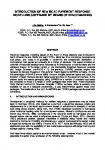
The model calibration process was applied to hot-mix asphalt concrete pavement (ACP) due to the availability of historical field data. It was less applicable to continuously reinforced concrete pavement (CRCP) and jointed plain concrete pavement (JPCP) due to limited availability of field data. Figure 3 shows an example calibrated model for Distress Score for pavement family A [thick ACP (PMIS Pavement Type 4), Intermediate ACP (PMIS Pavement Type 5), and overlaid ACP (PMIS Pavement Type 9)]. Heavy Rehab (HR)

Distres Score (DS)

100

Calibrated

80 60 40 20

Original

0 0

1

2

3

4

5

6

7

8

9

10 11 12 13 14 15

Age (years)

Figure 3. Calibrated and Original DS Prediction Models (Zone 1, Pavement Family A, & HR) (Number of data points (n)= 1647; Average 20-year ESALs = 4.74 million). OVERVIEW OF PMIS OPTIMIZATION PROCESS The PMIS optimization process is described in the PMIS Technical Manual published in December 2011 (TxDOT 2011). According to the technical manual, the optimization process consists of 10 steps; however six of them are the most critical: establishing distress quantities for the analysis base year, treatment selection from decision tress, “after treatment” distress ratings and ride quality, computation of benefits and effective life, cost effectiveness ratio calculations, and selection of pavement sections to be funded. The sequence of these critical steps is illustrated in Figure 4. Treatments considered in this process are categorized as PM, LR, MR, HR, and Needs Nothing (NN). The definitions of these treatment categories were discussed earlier in the previous section of this report. Predefined decision trees are used for identifying needed treatment category for each pavement section. Each treatment category is associated with a reason code as a function of seven factors: pavement type, distress ratings, Ride Score, average daily traffic per lane, functional class, average county rainfall, and time since last surfacing. These decision trees and associated reason codes are provided in PMIS technical manual.

5

Obtain Li for base year Obtain M/R treatments from decision trees Compute cost for M&R of each section Compute benefit for M&R for each section Compute cost effectiveness for each section Prioritize sections using ranking/optimization Figure 4. Flowchart of the Main Steps of PMIS’s Optimization Process. The effect of each treatment category on pavement performance is measured in terms of reduction in distress ratings and gain in ride score. Once a treatment category is selected, distress rating and ride score are adjusted according Table 1. The unit costs of these treatment categories may vary depending on local factors such as project location and size. The unit costs used in this study are shown in Table 1. Table 1. Condition Effects and Unit Costs for Treatment Categories Considered in PMIS Optimization Process. Treatment Gain in Distress Gain in Ride Unit Cost, $/lane-mile Category Utility Score (used in this study) Stop gap or need No change in distress No change in None nothing ratings Ride Score Reset distress ratings Increase Ride PM 29,000 to zero Score by 0.5 Reset distress ratings Increase Ride LR 173,000 to zero Score by 1.5 Reset distress ratings Increase Ride MR 237,000 to zero Score by 4.8 Reset distress ratings Increase Ride HR 442,000 to zero Score by 4.8 Benefits are measured as the area between the distress or ride utility curves before and after the suggested treatment is applied. Four possible scenarios for before and after utility curves are analyzed. • • • •

Curves intersect before the age of 20 years. Curves are parallel, in which case treatment life is set to 20 years. Curves approach each other very closely (a difference equal to or less than 0.0001 utility units), but they do not intersect. Curves reach the failure criterion of 0.6 distress utility and 0.3 ride utility.

6

According to the PMIS technical manual, the area is calculated using a trapezoidal approximation. In this investigation, the area between the before and after utility curves was calculated by integration using the following equation. 𝐴

𝐴𝑟𝑒𝑎𝑎𝑓𝑡𝑒𝑟 = ∫0 1 − 𝑒

𝜌𝑑 𝛽𝑑 � � 𝐴𝑔𝑒𝑑

�−�

𝑑𝑥 = 𝐴𝑔𝑒𝑑 −

𝛽𝑑 𝜌 1 ,� 𝑑 � � 𝛽𝑑 𝐴𝑔𝑒𝑑

𝜌𝑑 Γ�−

𝛽𝑑

(5)

To calculate the overall (or total) benefit, distress area (AD) and ride score area (AR) are added up considering equal weight for each one. In other words, total benefit (B) is computed using the following equation and with weights WD and WR set to 50. 𝑊

𝑊

𝐷 𝐵 = 2 �100 𝐴𝐷 + 100𝑅 𝐴𝑅 �

(6)

𝐿𝑀𝑥𝐵

(7)

The cost effectiveness ratio is calculated for each section based on the benefit of the selected treatment, treatment effective life (predicted using the performance prediction models discussed earlier), treatment uniform annual cost, section lane-miles, and vehicle miles traveled on the pavement section. The mathematical expression for computing this ratio is as follows:

CERatio LM B EffLife UACost

= = = = =

UACost TCost

= =

DRate InfRate n VMT

= = = =

𝐶𝐸𝑅𝑎𝑡𝑖𝑜 = 10000𝑥 �𝐸𝑓𝑓𝐿𝑖𝑓𝑒 𝑥 𝑈𝐴𝐶𝑜𝑠𝑡� 𝑥 𝑙𝑜𝑔10 𝑉𝑀𝑇

Cost-Effectiveness Ratio. Lane Miles. Benefit. Effective Life of the Needs Estimate treatment, in years. Uniform Annual Cost of the Needs Estimate treatment, in dollars. DRate(1 + DRate)EffLife UACost = TCost x � � (1 + DRate)Efflife − 1 Uniform Annual Cost of the Needs Estimate treatment, in dollars. Treatment Cost (current or future) of the Needs Estimate treatment TCost = UCostx(1 + InfRate)n Discount Rate, in percent per year; DRate=6.5%. Inflation Rate, in percent per year. Number of years that the Unit Cost has been projected. Vehicle Miles Traveled.

Finally the pavement sections are sorted in order of decreasing cost-effectiveness ratio. Sections are funded in this order until the available budget is depleted. Sections that are not selected to receive any treatment are classified as Stop Gap.

7

CHAPTER 2 FEEDBACK FROM TXDOT PRACTITIONERS ON NEWLY DEVELOPED PAVEMENT PERFORMANCE PREDICTION MODELS Two webinars on the newly-developed performance prediction models were conducted for TxDOT practitioners from various districts throughout the state. The webinars provided an overview of the mathematical forms, calibration process, and sensitivity and accuracy of these models. The first webinar covered the ACP performance prediction models. The second webinar covered the continuously reinforced concrete pavement (CRCP) and jointed concrete pavement (JCP) prediction models. The webinar presentations are contained in Product 5-6386-01-P1. ACP PERFORMANCE PREDICTION MODELS Following the introductory webinar for the ACP performance prediction models, a series of webbased surveys were prepared and launched to obtain feedback from TxDOT’s practitioners on the reasonableness and accuracy of the ACP prediction curves based on their practical experiences. To account for differences in pavement performance among the different climate-subgrade zones of TxDOT’s districts, a separate survey was conducted for each zone, with a total of four surveys. Each of the four web surveys presented the developed performance prediction curves in several ways so that the participants can evaluate the reasonableness of the developed curves under different combinations of pavement type, M&R type, and traffic level. Specifically, within each survey (one survey for each of the four climate-subgrade zones), and for each pavement family (there are three pavement families), the following figures are presented to the respondents: First, the web survey starts with four figures (for four different M&R types) consisting of the performance prediction curves of pavements with similar type, M&R treatment, and subgradeclimate, but different traffic levels. Each one of these figures includes three curves (for three different traffic levels) as well as the original performance curve. These figures are used to: (1) show how the models account for the effect of traffic level on pavement deterioration, and (2) compare the new curves with original ones. Figure 5 is an example of these figures.

Figure 5. Example Figure from Web Survey Showing How the Models Account for the Effect of Traffic Level on Pavement Deterioration after Applying Heavy Rehabilitation to Pavement Family A in Zone 1. 9

Second, the web survey has three figures consisting of the ACP performance prediction curves of pavements with similar pavement family, traffic level, and subgrade-climate, but different M&R treatment. These figures are used to: (1) show how the models account for the effect of M&R type on pavement deterioration, and (2) compare the developed curves with original ones. Figure 6 is an example of these figures.

Figure 6. Example Figure from Web Survey Showing How the Models Account for the Effect of M&R Type on Pavement Deterioration (Pavement Family A in Zone 1). Third, the web survey ends with 12 figures (for all combinations of four M&R types and three traffic levels) consisting of the utility curves of each individual ACP distress type. These curves are used to show how the models account for the contribution of each individual distress type on pavement deterioration. Figure 7 is an example of these figures.

10

Figure 7. Example Figure from Web Survey Showing How the Models Account for the Contribution of Each Individual Distress Type on Pavement Deterioration (Zone 1, Pavement Family B, and Medium Traffic). In some cases, some curves have not been developed due to the lack of historical condition data and thus were not presented in the survey. The four web surveys are presented in Appendix A. ACP MODEL SURVEY RESULTS AND FOLLOW-UP EFFORTS A total of 17 survey responses were received for the ACP models, including five responses from Zone 1, four responses from Zone 2, six responses from Zone 3, and two responses from Zone 4. These responses are from transportation and pavement engineers and managers from the districts of Abilene, Brownwood, Bryan, Childress, Corpus Christi, Dallas, Fort Worth, Lubbock, Odessa, Paris, and Wichita Falls. As can be seen from Figure 8, a large majority of all responses (93 percent) rated the performance curves as either reasonable or slightly over or under predicting. This suggests that, in most cases, the respondents believe that the model predictions of pavement condition agree with or slightly differ from their own experience. Only 7 percent of all responses indicated that the models predictions are unreasonable (i.e., highly over or under predict pavement condition). This suggests that only in a few cases the respondents believe that the model predictions of pavement condition are considerably lower or higher than their own experience. These cases are shown in Table 2. 11

17%

4% 3%

16% Highly Overpredicts Slightly Overpredicts Reasonable Slightly Underpredicts

60%

Highly Underpredicts

Figure 8. Opinions of TxDOT’s Practitioners of Newly-Developed Pavement Performance Prediction Models. Almost all of the “highly over/under predicting” responses are from the three districts of Paris, Bryan, and Brownwood. Within these cases, the Paris District responses suggest that the models predictions are highly optimistic; the Brownwood District responses suggest that the models predictions are highly pessimistic; and the Bryan District responses are mixed (suggesting that the models are highly optimistic in some cases and highly pessimistic in other cases). Follow-up phone calls were made to the respondents who indicated that at least one curve highly over/under predicts pavement performance. They were asked to specify example roadway segments that, in their opinion, represent the typical pavement performance in their districts for certain combinations of climate, subgrade, traffic, pavement type, and M&R history. The researchers extracted the historical pavement condition data for these typical roadway segments from PMIS and compared it to the condition data predicted by the new models. Table 3 presents the provided typical roadway segment. Historical pavement condition data (i.e., DS) of the specified segments were extracted from PMIS database. Their M&R and construction data were extracted from TxDOT’s Design and Construction Information System (DCIS) database. The extracted condition data are then plotted versus their corresponding prediction curves and presented in Figures 8 through 20. Each point in the graphs represents the average DS of all PMIS sections that compose the specified segment. As can be seen from these figures, the actual condition data for most of the typical segments match the models predictions reasonably.

12

Table 2. Summary of Responses Indicating Highly over or under Prediction of Pavement Condition by the New Models. Zone 1 1 1 1 1 1 1 1

Performance Curve Pavement M&R Family Type A MR A HR A HR A HR B PM B LR B MR B HR

Response Traffic

Model Rating

District

Low Low Medium High Medium Medium Medium Medium

Highly Overpredicts Highly Overpredicts Highly Overpredicts Highly Overpredicts Highly Overpredicts Highly Overpredicts Highly Overpredicts Highly Overpredicts

Paris Paris Paris Paris Paris Paris Paris Paris Corpus Christi Bryan Bryan Bryan Bryan Bryan Bryan Brownwood Brownwood Brownwood Brownwood Brownwood Brownwood Brownwood Brownwood

2

A

MR

Low

Highly Underpredicts

2 2 2 2 2 2 3 3 3 3 3 3 3 3 3 3

B B B B B B A A A A A A A B B B

PM PM LR LR MR MR HR HR PM PM PM LR MR PM LR HR

Low Medium Low Medium Low Medium Medium High Low Medium High High High Low Low Low

Highly Underpredicts Highly Underpredicts Highly Underpredicts Highly Underpredicts Highly Underpredicts Highly Underpredicts Highly Overpredicts Highly Overpredicts Highly Underpredicts Highly Underpredicts Highly Underpredicts Highly Underpredicts Highly Underpredicts Highly Underpredicts Highly Underpredicts Highly Underpredicts

13

Table 3. Roadway Segments Provided by the Respondents as Representative of Typical Performance. District Paris Paris Paris Bryan Bryan Corpus Christi Corpus Christi Brownwood Brownwood Brownwood Brownwood Brownwood Abilene Odessa Odessa Odessa Odessa

County Delta Lamar Fannin Brazos County Madison

Highway Name SH-24 FM-195 SH-121 US-190 I-45

BRM 218 658 210 686 134

ERM 224 668 216 692 152

San Patricio

FM-2986

602

604

San Patricio

SH-188

538

570

Eastland Lampasas Coleman Brown McCulloch Scurry Midland Reeves Martin Pecos

IH-20 US190 US-84 US-84 US190 US-84 IH-20 IH-10 SH-349 BI-10G

333 540 520 568 460 384 122 204 288 236

340 550 528 574 468 426 136 209 344 455

Distress Score (DS)

100 80 60 40 20 0

1

2

3

4

5

6

7

8

9

Age (years)

10 11 12 13 14 15

Figure 9. Actual vs. Predicted DS (Zone 1, Pavement Family A, Low Traffic, PM).

14

100

Distress Score (DS)

80 60 40 20 0

1

2

3

4

5

6

7

8

Age (years)

9

10

11

12

13

14

15

Figure 10. Actual vs. Predicted DS (Zone 1, Pavement Family A, Medium Traffic, PM). 100

Distress Score (DS)

80 60 40 20 0

1

2

3

4

5

6

7

8

9 10 11 12 13 14 15 16 17 18 19 20 Age (years)

Figure 11. Actual vs. Predicted DS (Zone 2, Pavement Family A, Medium Traffic, PM).

Distress Score (DS)

100 80 60 40 20 0

1

2

3

4

5

6

7

8

9

10

11

12

13

14

15

Age (years)

Figure 12. Actual vs. Predicted DS (Zone 2, Pavement Family C, Medium Traffic, PM). 15

Distress Score (DS)

100 80 60 40 20 0

1

2

3

4

5

6

7

8

Age (years)

9

10

11

12

13

14

15

Figure 13. Actual vs. Predicted DS (Zone 3, Pavement Family A, Medium Traffic, PM).

Distress Score (DS)

100 80 60 40 20 0

1

2

3

4

5

6

7

8

Age (years)

9

10

11

12

13

14

15

Figure 14. Actual vs. Predicted DS (Zone 3, Pavement Family A, Medium Traffic, MR). 100

Distress Score (DS)

80 60 40 20 0

1

2

3

4

5

6

7

8

9

10

11

12

13

14

15

Age (years)

Figure 15. Actual vs. Predicted DS (Zone 3, Pavement Family A, High Traffic, PM).

16

100

Distress Score (DS)

80 60 40 20 0

1

2

3

4

5

6

7

8

Age (years)

9

10

11

12

13

14

15

Figure 16. Actual vs. Predicted DS (Zone 3, Pavement Family A, High Traffic, MR). 100

Distress Score (DS)

80 60 40 20 0

1

2

3

4

5

6

7

8

9

Age (years)

10

11

12

13

14

15

Figure 17. Actual vs. Predicted DS (Zone 3, Pavement Family A, High Traffic, HR).

Distress Score (DS)

100 80 60 40 20 0

1

2

3

4

5

6

7 8 Age (years)

9

10

11

12

13

14

15

Figure 18. Actual vs. Predicted DS (Zone 3, Pavement Family C, Medium Traffic, PM). 17

Distress Score (DS)

100 80 60 40 20 0

1

2

3

4

5

6

8 9 Age7 (years)

10

11

12

13

14

15

Figure 19. Actual vs. Predicted DS (Zone 3, Pavement Family C, Medium Traffic, MR).

Distress Score (DS)

100 80 60 40 20 0

1

2

3

4

5

6

7

8

9

Age (years)

10

11

12

13

14

15

Figure 20. Actual vs. Predicted DS (Zone 4, Pavement Family C, Low Traffic, PM).

Distress Score (DS)

100 80 60 40 20 0

1

2

3

4

5

6

7

8

Age (years)

9

10

11

12

13

14

15

Figure 21. Actual vs. Predicted DS (Zone 4, Pavement Family C, High Traffic, LR).

18

CRCP AND JCP PERFORMANCE PREDICTION MODELS The second webinar presented the CRCP and JCP performance prediction models to TxDOT personnel that had experience with these pavement types. The webinar presentations are contained in Product 5-6386-01-P1. The general consensus among TxDOT participants in that webinar was that the models as presented did not need any changes at this time. However, in the future, TxDOT personnel indicated that coarse aggregate type be included for the CRCP performance prediction models in the future, since CRCP performance is affected by coarse aggregate type. Currently, the PMIS database does not contain coarse aggregate type for CRCP. In addition, TxDOT personnel indicated that JCP performance is highly dependent on variations in subgrade and environmental conditions. In addition, several participants indicated problems with JCP that had no load transfer devices (i.e., poor load transfer efficiency) or poor subbase support. Currently, the PMIS database does not contain load transfer or subbase support information for JCP.

19

CHAPTER 3 EVALUATION OF PMIS OPTIMIZATION PROCESS This chapter provides an evaluation of the logic of the PMIS optimization process. This process was programmed in a spreadsheet (called “replicate” henceforth) and the results of this replicate were compared to the output of PMIS. The replicate spreadsheet includes all of the optimization process steps described in the PMIS Technical Manual (TxDOT 2011). The evaluation was conducted using data from the Bryan District and was divided into three stages, as illustrated in Figure 22. Start Obtain Li for Base Year Obtain needed M&R Treatments from Decision Trees

Evaluation Stages Stage 2

Stage 1

Stage 3

• Obtain latest available Li values from PMIS • Test need analysis for 2011

Compute M&R Cost for each Section

• Obtain latest available Li values from PMIS • Test remaining steps

Compute M&R Benefit for each Section Compute Cost Effectiveness Ratio for each Section • Obtain needed M&R, benefit, and cost from PMIS output for 20112014 • Evaluate ranking step

Prioritize sections using ranking/optimization

Figure 22. Illustration of PMIS Optimization Process and Evaluation Stages. Figure 23 shows the needed and funded M&R investments (obtained from PMIS output) for the years 2011–2014 for Bryan District. The funded investments were used as annual budgets in the replicate. While the analysis was done for a 10-year period, only the results of the first four years (2011–2014) are presented here for simplicity and to be consistent with TxDOT approach of developing 4-year pavement management plans. Table 4 shows the allocations of these investments among the four treatment categories (PM, LR, MR, and HR), as determined by PMIS.

21

70.0

Amount, M$

60.0 50.0 40.0

Needed

30.0

Funded

20.0 10.0 0.0

2011

2012

2013

2014

Figure 23. Needed and Funded Investments for Bryan District, Obtained from PMIS (in Million Dollars). STAGE 1: EVALUATION OF THE NEEDS ANALYSIS STEP The purpose of this stage is to evaluate the needs analysis component of the optimization process by comparing the needed treatments in 2011 (obtained from PMIS output) to those obtained from the replicate. Table 4 presents the agreements and differences between PMIS and the replicate in terms of needed lane-miles of each treatment category in 2011. For example, PMIS and the replicate agree on 766 lanes-miles of PM; but differ on one lane-mile (identified by PMIS as “needs PM” and by the replicate as “needs LR”). This one lane-mile discrepancy is located on FM0179 (MR 246+02.0 to 246+01.5). This section’s Ride Score in 2011 was 2.447. According to the decision tree reason code A200, this section needs LR (since Ride Score is less than 2.5); but PMIS indicates that it does not need any M&R action. As can be seen from Table 4, there are minor differences between PMIS and the replicate in terms treatments identified by the needs analysis. Most of these discrepancies occur in sections that are classified by PMIS as “Need Nothing” but classified by the replicate as PM, and ones that are classified by PMIS as LR but classified by the replicate as MR. This suggests that PMIS may not be adhering strictly to the decision trees (documented in the PMIS technical manual). Table 4. Lane-Miles of Treatment According to PMIS and Replicate Needs Analyses for 2011. According to Replicate PM LR MR HR NN PM 766 1.0 LR 20.1 4.0 According to MR 96.9 1.0 PMIS HR 25.4 NN 3.4 1 0 0 1,001.9 22

STAGE 2: EVALUATION OF THE RANKING STEP The purpose of this stage is to evaluate the ranking step of the optimization process. The needed treatments, predicted performance, and cost-effectiveness calculations are obtained directly from the PMIS output. Thus, any differences between the PMIS output and the replicate spreadsheet output can be attributed to differences in the ranking step (i.e., prioritizing pavement sections that need M&R treatment based on their cost-effectiveness ratio). As can be seen from Figures 24 and 25, PMIS and the replicate agree in terms of allocated funds and lane-miles of each treatment category. Minor differences can be attributed to minor simplifying assumptions that were made in the replicate spreadsheets. This suggests that the ranking step of the optimization process is coded properly in PMIS. 18 16

Amount, M$

14 12 10

PMIS

8

Replicate

6 4 2 0

PM

LR

MR

HR

Figure 24. Investment in Funded Projects within Each Treatment Category for Bryan District in 2011 (in Million Dollars). 250

Lane-miles

200 150

PMIS

100

Replicate

50 0

PM

LR

MR

HR

Figure 25. Lane-Miles of Each Treatment Category in 2011 (Bryan District).

23

STAGE 3: EVALUATION OF THE OPTIMIZATION PROCESS AS A WHOLE The purpose of this stage is to evaluate the optimization process as a whole. As can be seen from Figures 26, noticeable differences exist between PMIS and the replicate in terms of total allocated funds for LR and HR over the 2011–2014 period. These differences between PMIS and the replicate exist in all treatment categories when these funds are evaluated on a year-by-year basis (see Table 5). A similar pattern exists in terms of lane-miles of each treatment category (Figure 27 and Table 6). 30

Total M$

25 20 PMIS

15

Replicate

10 5 0

PM

LR

MR

HR

Figure 26. PMIS and Replicated Total Funded Projects in 4 Years (in Million Dollars). Table 5. Funds Allocation from PMIS Output and Replicate in (in Million Dollars). Year PM LR MR HR PMIS Rep. PMIS Rep. PMIS Rep. PMIS Rep. 2011 Needed 22.2 22.3 4.2 3.8 23.3 24.0 11.2 11.9 5.9 6.2 0.0 2.6 16.1 12.8 4.1 4.5 Funded 2012 Needed 17.3 8.3 0.7 0.1 2.0 4.4 5.7 0.4 8.8 8.3 0.3 0.1 0.5 4.4 5.6 0.4 Funded 2013 Needed 8.6 9.4 1.3 0.0 5.6 0.0 0.2 0.4 3.4 4.4 0.4 0.0 0.5 0.0 0.1 0.0 Funded 2014 Needed 5.2 14.6 3.8 0.9 8.8 0.0 7.4 0.4 2.4 8.5 0.0 0.0 6.1 0.0 0.0 0.0 Funded

24

1000 900

Total Lane-miles

800 700 600 500

PMIS

400

Replicate

300 200 100 0

PM

LR

MR

HR

Figure 27. PMIS and Replicate Total Lane-Miles of Each Treatment Category for 4 Years. Table 6. PMIS Output and Replicate Yearly Lane-Miles of Each Treatment Category. PM 2011 2012 2013 2014

PMIS 203 302 117 83

LR Rep. 214 268 141 282

PMIS 0 2 2 0

MR Rep. 15 1 0 0

PMIS 68 2 2 26

HR Rep. 54 18 0 0

PMIS 9 13 0 0

Rep. 10 1 0 0

In both outputs (PMIS and replicate) the funded pavement sections are predominantly PM. This behavior may be explained by (a) the limited influence that “effective life” has on the costeffectiveness ratio (Note that effective life affects both the numerator and denominator of the equation of the cost-effectiveness ratio, which diminishes its effect), and (b) the relative benefit differences and the relative cost differences among these four treatment categories. Table 7 shows the unit costs, annual benefit, annual cost, and CERatio for the four treatment categories for an example pavement section (Highway BS0011H, Beginning Reference Marker 336, 0.3-mile long, 4 lanes, and ADT of 3,400 vehicles per day). The rehabilitation categories (LR, MR and HR) have much higher unit costs and uniform annual costs compared to the PM category. Thus, to be selected by the optimization procedure (i.e., to have higher CERatio), these rehabilitation categories must have very high benefits. For example, for HR to be selected over PM in this case, its benefit must be at least 10.2 times the benefit of PM. This explains the predominant selection of PM compared to the rehabilitation categories. The implication of this observation is that PMIS’s optimization process appears to favor low-cost treatments over long- life treatments.

25

Table 7. Comparison of Benefit and Cost Parameters for the Four Treatment Categories for an Example Pavement Section. Attribute Unit Cost, $/lane mile Uniform Annual Cost, $ Annual Benefit Effective Life, years VMT CERatio

PM 29,000 47.06 3,803.02 11 372,300 123.74

LR 173,000 47.72 20,102.68 13 372,300 23.74

MR 237,000 47.86 25,004.78 15 372,300 19.14

HR 442,000 53.69 44,445.23 17 372,300 12.08

Table 8 shows the average Distress Score, Ride Score, and Condition Score after the selected treatments are applied in each year. As can be seen from this table, PMIS and the replicate agree in terms of average condition of the network for all indicators. Minor differences between PMIS and the replicate in terms of these indexes averages can be explained by minor discrepancies in the needs analysis (see discussion of Stage 2), minor simplifying assumptions used in the replicate, and discrepancies in the Ride Score performance prediction models. Table 8. Average Distress, Ride and Condition Scores from PMIS Output and Replicate. PMIS Replicate Year DS Ride CS DS Ride CS 2011 89.85 3.66 87.31 89.85 3.65 87.31 2012 93.78 4.61 92.21 97.23 4.41 90.89 2013 95.76 4.32 94.33 97.96 4.33 96.16 2014 96.60 4.28 94.56 97.32 4.25 93.33

26

CHAPTER 4 SUMMARY AND FINDINGS The research team presented the ACP, CRCP, and JCP performance prediction models to TxDOT personnel through two webinars and an ACP model web survey. The researchers also evaluated the logic and output of PMIS optimization process. ACP PERFORMANCE PREDICTION MODELS Following the webinar for the ACP performance prediction models, a series of web-based surveys were prepared and launched to obtain feedback from TxDOT’s practitioners on the reasonableness and accuracy of the ACP prediction curves based on their practical experiences. To account for differences in pavement performance among the different climate-subgrade zones of TxDOT’s districts, a separate survey was conducted for each zone, with a total of four surveys. A total of 17 survey responses were received for the ACP models from the Abilene, Brownwood, Bryan, Childress, Corpus Christi, Dallas, Fort Worth, Lubbock, Odessa, Paris, and Wichita Falls Districts. A large majority of all responses (93 percent) rated the performance curves as either reasonable or slightly over or under predicting. Only 7 percent of all responses indicated that the models predictions are unreasonable (i.e., highly over or under predict pavement condition). Almost all of the “highly over/under predicting” responses are from the Paris, Bryan, and Brownwood Districts. Follow-up phone calls were made to the respondents who indicated that at least one curve highly over/under predicts pavement performance. They were asked to specify example roadway segments that, in their opinion, represent the typical pavement performance in their districts for certain combinations of climate, subgrade, traffic, pavement type, and M&R history. The researchers extracted the historical pavement condition data for these typical roadway segments from PMIS and compared it to the condition data predicted by the new models. The actual condition data for most of these segments match the model predictions. Based on the above findings, the research team concluded that the ACP pavement performance prediction models do not need modification at this time. Appendix B contains the ACP performance model coefficients. CRCP AND JCP PERFORMANCE PREDICTION MODELS The second webinar presented the CRCP and JCP performance prediction models to TxDOT personnel that had experience with these pavement types. The general consensus among TxDOT participants in that webinar was that the models as presented did not need any changes at this time. However, in the future, TxDOT personnel indicated that coarse aggregate type should be included for the CRCP performance prediction models in the future, since CRCP performance is affected by coarse aggregate type. Currently, the PMIS database does not contain coarse aggregate type for CRCP. TxDOT personnel indicated that JCP performance is highly dependent on variations in subgrade and environmental conditions. In addition, several participants indicated problems with JCP that had no load transfer devices (i.e., poor load transfer efficiency) or poor subbase support. 27

Currently, the PMIS database does not contain load transfer or subbase support information for JCP. Appendix C contains the CRCP performance model coefficients. Appendix D contains the JCP performance model coefficients. EVALUATION OF THE PMIS OPTIMIZATION PROCESS The research team also evaluated the logic of the PMIS optimization process. This process was programmed in a spreadsheet (called replicate) and the results of this replicate were compared to the output of PMIS. The replicate spreadsheet includes all of the optimization process steps described in the PMIS Technical Manual (TxDOT 2011). The evaluation was conducted using data from the Bryan district. PMIS and the replicate were found to agree in terms of M&R treatments, needed and allocated budgets, and condition indicators in the first year of the planning period. However, minor differences began to appear and accumulate in future years of the planning period. These differences can be explained by minor discrepancies in the needs analysis, minor simplifying assumptions used in the replicate, and discrepancies in the Ride Score performance prediction models. In both outputs (PMIS and replicate) the funded pavement sections are predominantly PM. This behavior may be explained by (a) the limited influence that “effective life” has on the costeffectiveness ratio, and (b) the relative benefit differences and the relative cost differences among these four treatment categories. The implication of this observation is that PMIS’s optimization process appears to favor low-cost treatments over long- life treatments.

28

REFERENCES Gharaibeh, N., T. Freeman, S. Saliminejad, C. Chang-Albitres, J. Weissman, A. Weissman, A. Wimsatt, and C. Gurganus (2012). Evaluation and Development of Pavement Scores, Performance Models and Needs Estimates for the TxDOT Pavement Management Information System. Final Report No. FHWA/TX-12/0-6386-3, Texas Transportation Institute, Texas A&M University System, College Station, Texas, 2012. Murphy, M. and Zhang, Z. (2009). Assumptions Used in Selecting Project Class (PMIS Treatment Types) for the District 4-year Pavement Management Plans. Draft Report to TxDOT. Stampley, B. E., Miller, B., Smith, R. E., and Scullion, T. (1995). Pavement Management Information System Concepts, Equations, and Analysis Models. Report No. TX-96/1989-1, Texas Transportation Institute and Texas Department of Transportation. TxDOT (2011). PMIS Technical Manual. Prepared by Texas Department of Transportation Construction Division, Materials and Pavements Section, December 2011.

29

APPENDIX A: WEB SURVEY

A-1

Qualtrics Survey Software

1 of 24

https://dc-viawest.qualtrics.com/ControlPanel/PopUp.php?PopType=Sur...

TxDOT Project

Calibration of PMIS Pavement Performannce Prediction Models Conducted as part of TxDOT Project 0-6386

Zone 1

General

General Q1. Please provide your contact information below: Name (required) District Title E-mail Pvt Family A

Definitions Zone 1: wet-cold climate, and poor, very poor, or mixed subgrade

Pavement Family A: •Thick ACP (PMIS Pavement Type 4) •Intermediate ACP (PMIS Pavement Type 5) •Overlaid ACP (PMIS Pavement Type 9) Age0:The age when distress first appears Age70:The age when DS drops into 70 8/17/2012 3:29 PM


2 of 24


DS15:DS at the age of 15 years Low Traffic: 20-year projected cumulative ESAL of lass than 1.0 million ESALs. Medium Traffic: 20-year projected cumulative ESAL of between1.0 million and 10 million ESALs. High Traffic: 20-year projected cumulative ESAL of higher than 10 million ESALs.

Performance Curves for Zone 1, Pvt Family A, and Preventive Maintenance (PM)

Q2. Please rate the above curves as follows: Highly Overpredicts (The curve should be shifted down or left)

Slightly Overpredicts (The curve should be shifted down or left)

Reasonable

Slightly Undepredicts (The curve should be shifted up or right)

Highly Undepredicts (The curve should be shifted up or right)

Low Traffic Medium Traffic High Traffic

Comments:

8/17/2012 3:29 PM


3 of 24


Performance Curves for Zone 1, Pvt Family A, and Light Rehabilitation (LR)



Reasonable




Comments:

8/17/2012 3:29 PM


4 of 24


Performance Curves for Zone 1, Pvt Family A, and Medium Rehabilitation (MR)



Reasonable




Comments:

8/17/2012 3:29 PM


5 of 24


Performance Curves for Zone 1, Pvt Family A, and Heavy Rehabilitation (HR)



Reasonable




Comments:

Comparison of Zone1 and Pavement Family A Models Grouped by Treatment Types and Traffic Levels

8/17/2012 3:29 PM


6 of 24


Q6. Please review the above curves and provide any comments you might have.

Comparison of Utility Curves for Various Distresses (Grouped by Treatment Types) for Zone 1, Pavement Family A and Low Traffic

8/17/2012 3:29 PM


7 of 24



Comparison of Utility Curves for Various Distresses (Grouped by Treatment Types) for Zone 1, Pavement Family A and Medium Traffic

8/17/2012 3:29 PM


8 of 24



Comparison of Utility Curves for Various Distresses (Grouped by Treatment Types) for Zone 1, Pavement Family A and High Traffic

8/17/2012 3:29 PM


9 of 24



Pvt Family B


8/17/2012 3:29 PM


10 of 24


Pavement Family B: •Composite pavement (PMIS Pavement Type 7) •Concrete pavement overlaid with ACP (PMIS Pavement Type 8) Age0:The age when distress first appears Age70:The age when DS drops into 70 DS15:DS at the age of 15 years Low Traffic: 20-year projected cumulative ESAL of lass than 1.0 million ESALs. Medium Traffic: 20-year projected cumulative ESAL of between1.0 million and 10 million ESALs. High Traffic: 20-year projected cumulative ESAL of higher than 10 million ESALs.

Performance Curves for Zone 1, Pvt Family B, and Preventive Maintenance (PM)



Reasonable




Comments:

8/17/2012 3:29 PM


11 of 24


Performance Curves for Zone 1, Pvt Family B, and Light Rehabilitation (LR)



Reasonable




Comments:

8/17/2012 3:29 PM


12 of 24


Performance Curves for Zone 1, Pvt Family B, and Medium Rehabilitation (MR)



Reasonable




Comments:

8/17/2012 3:29 PM


13 of 24


Performance Curves for Zone 1, Pvt Family B, and Heavy Rehabilitation (HR)



Reasonable




Comments:

Comparison of Zone 1 and Pavement Family B Models Grouped by Treatment Types and Traffic Levels

8/17/2012 3:29 PM


14 of 24



Comparison of Utility Curves for Various Distresses (Grouped by Treatment Types) for Zone 1, Pavement Family B and Low Traffic

8/17/2012 3:29 PM


15 of 24



Comparison of Utility Curves for Various Distresses (Grouped by Treatment Types) for Zone 1, Pavement Family B and Medium Traffic

8/17/2012 3:29 PM


16 of 24



Comparison of Utility Curves for Various Distresses (Grouped by Treatment Types) for Zone 1, Pavement Family B and High Traffic

8/17/2012 3:29 PM


17 of 24



Pvt Family C


8/17/2012 3:29 PM


18 of 24


Pavement Family C: •Thin ACP (PMIS Pavement Type 6) •Thin-surfaced ACP (PMIS Pavement Type 10) Age0:The age when distress first appears Age70:The age when DS drops into 70 DS15:DS at the age of 15 years Low Traffic: 20-year projected cumulative ESAL of lass than 1.0 million ESALs. Medium Traffic: 20-year projected cumulative ESAL of between1.0 million and 10 million ESALs. High Traffic: 20-year projected cumulative ESAL of higher than 10 million ESALs.

Performance Curves for Zone 1, Pvt Family C, and Preventive Maintenance (PM)

Q18. Please rate the above curves as follows: Note that the models for medium and high traffic are not developed due to insufficient data. Highly Overpredicts (The curve should be shifted down or left)


Reasonable



Low Traffic

Comments:

8/17/2012 3:29 PM


19 of 24


Performance Curves for Zone 1, Pvt Family C, and Light Rehabilitation (LR)

Q19. Please rate the above curves as follows: Note that the models for medium and high traffic are not developed due to insufficient data.

Highly Overpredicts (The curve should be shifted down or left)


Reasonable



Low Traffic

Comments:

8/17/2012 3:29 PM


20 of 24


Performance Curves for Zone 1, Pvt Family C, and Medium Rehabilitation (MR)




Reasonable



Low Traffic

Comments:

8/17/2012 3:29 PM


21 of 24


Performance Curves for Zone 1, Pvt Family C, and Heavy Rehabilitation (HR)




Reasonable



Low Traffic

Comments:

Comparison of Zone 1 and Pavement Family C Models Grouped by Treatment Types and Traffic Levels

8/17/2012 3:29 PM


22 of 24


Q22. Please review the above curves and provide any comments you might have. Note that the models for medium and high traffic are not developed due to insufficient data.

Comparison of Utility Curves for Various Distresses (Grouped by Treatment Types) for Zone 1, Pavement Family C and Low Traffic

8/17/2012 3:29 PM


23 of 24



Q24. Please provide the information of the candidate roadway section(s) that can be used for improving the models: Section 1

Section 2

Section 3

Section 4

Section 5

County Name Highway Name Beginning Reference Marker Ending Reference Marker

Comments:

Q25. Please provide the suggestions you might have on the groups with insufficient data.

Submit

By clicking on the Next button, your responses will be submitted and the survey ends here.

8/17/2012 3:29 PM


24 of 24


8/17/2012 3:29 PM

APPENDIX B CALIBRATED ACP PERFORMANCE MODEL COEFFICIENTS NOTE: For the following tables, Low Traffic is defined as having a projected 20 year 18KESAL forecast below 1,000,000; Medium Traffic is between 1,000,000 and 10,000,000; and High Traffic is greater than or equal to 10,000,000.

B-1

Calibrated model coefficients for Zone 1-pavement family A Low Traffic Distress Type

Shallow Rutting

Deep Rutting

Failures

Block Cracking

Alligator Cracking

Longitudinal Cracking

Transverse Cracking

Patching

Ride Score

Medium Traffic

High Traffic

Treatment Type

α

β

A

α

β

A

α

β

A

PM

100.00

0.41

75.16

100.00

0.43

102.38

100.00

0.39

58.34

LR

100.00

0.47

79.75

100.00

0.47

107.18

100.00

0.42

66.85

MR

100.00

0.52

80.38

100.00

0.55

121.09

100.00

0.47

67.14

HR

100.00

0.53

91.69

100.00

0.58

122.99

100.00

0.55

70.69

PM

100.00

0.54

88.24

100.00

0.76

60.35

100.00

0.58

95.02

LR

100.00

0.55

101.18

100.00

0.80

68.37

100.00

0.60

113.20

MR

100.00

0.56

115.81

100.00

0.88

80.79

100.00

0.65

116.07

HR

100.00

0.57

133.23

100.00

1.01

83.07

100.00

0.73

123.10

PM

20.00

1.11

23.48

20.00

1.30

19.85

20.00

3.61

8.86

LR

20.00

1.17

24.55

20.00

1.33

20.51

20.00

3.88

9.10

MR

20.00

1.26

27.30

20.00

1.37

21.50

20.00

4.19

9.14

HR

20.00

1.40

30.05

20.00

1.40

21.49

20.00

4.54

9.18

PM

100.00

3.73

114.51

100.00

0.96

45.92

100.00

6.75

83.46

LR

100.00

3.81

130.91

100.00

1.83

47.93

100.00

7.69

94.98

MR

100.00

4.46

142.20

100.00

2.58

48.74

100.00

8.80

108.82

HR

100.00

4.98

146.76

100.00

3.14

58.32

100.00

10.10

125.49

PM

100.00

0.58

101.42

100.00

0.49

96.93

100.00

4.24

8.20

LR

100.00

0.62

104.61

100.00

0.53

113.11

100.00

5.10

9.67

MR

100.00

0.72

115.98

100.00

0.58

133.61

100.00

5.73

11.28

HR

100.00

0.73

135.90

100.00

0.65

159.49

100.00

6.06

11.90

PM

500.00

0.52

116.51

500.00

0.53

90.24

500.00

0.44

69.52

LR

500.00

0.60

133.63

500.00

0.54

104.52

500.00

0.50

71.55

MR

500.00

0.67

146.86

500.00

0.56

123.32

500.00

0.51

81.25

HR

500.00

0.71

153.66

500.00

0.59

146.45

500.00

0.58

84.37

PM

20.00

0.71

95.12

20.00

0.49

68.47

20.00

0.88

20.33

LR

20.00

1.11

109.50

20.00

0.54

68.87

20.00

0.92

21.07

MR

20.00

1.52

125.33

20.00

0.55

77.01

20.00

0.99

22.61

HR

20.00

1.95

143.04

20.00

0.61

78.23

20.00

1.09

25.68

PM

100.00

0.38

101.23

100.00

0.64

49.65

100.00

0.52

87.67

LR

100.00

0.41

105.68

100.00

0.65

53.60

100.00

0.52

100.95

MR

100.00

0.48

119.25

100.00

0.65

57.65

100.00

0.53

115.41

HR

100.00

0.50

119.67

100.00

0.78

61.64

100.00

0.54

131.59

PM

100.00

2.27

8.69

100.00

2.09

9.74

100.00

3.68

8.45

LR

100.00

4.46

10.48

100.00

2.41

10.16

100.00

6.47

11.14

MR

100.00

4.96

14.69

100.00

2.47

14.96

100.00

8.83

12.93

HR

100.00

42.52

18.71

100.00

44.12

19.52

100.00

47.08

18.53

B-

Calibrated model coefficients for Zone 1-pavement family B

Distress Type Shallow Rutting

Deep Rutting

Failures

Block Cracking

Alligator Cracking


Transverse Cracking

Patching

Ride Score

Low Traffic

Medium Traffic

High Traffic

Treatment Type

α

β

A

α

β

A

α

β

A

PM

100.00

0.39

90.81

100.00

0.73

51.56

100.00

0.30

99.51

LR

100.00

0.41

106.60

100.00

0.74

56.02

100.00

0.33

103.93

MR

100.00

0.43

127.73

100.00

0.75

60.38

100.00

0.38

115.99

HR

100.00

0.46

130.80

100.00

0.76

64.74

100.00

0.39

137.75

PM

100.00

0.60

101.99

100.00

0.73

82.60

100.00

0.51

101.42

LR

100.00

0.67

121.58

100.00

0.86

91.14

100.00

0.58

120.33

MR

100.00

0.78

124.74

100.00

0.98

96.09

100.00

0.68

122.26

HR

100.00

0.94

131.24

100.00

1.08

97.65

100.00

0.83

127.33

PM

20.00

0.42

118.33

20.00

0.68

97.50

20.00

0.57

109.25

LR

20.00

0.62

129.27

20.00

0.72

98.24

20.00

1.18

126.57

MR

20.00

0.66

153.80

20.00

0.79

102.39

20.00

1.71

144.27

HR

20.00

0.89

167.58

20.00

0.90

110.55

20.00

2.12

160.90

PM

100.00

0.63

118.81

100.00

3.89

50.61

100.00

7.79

25.39

LR

100.00

0.80

133.78

100.00

4.21

55.19

100.00

9.31

26.85

MR

100.00

0.90

140.54

100.00

4.58

59.86

100.00

9.62

29.82

HR

100.00

1.18

165.32

100.00

4.99

65.57

100.00

10.32

34.55

PM

100.00

0.46

74.29

100.00

0.54

53.38

100.00

3.34

9.15

LR

100.00

0.53

78.08

100.00

0.56

58.71

100.00

3.64

9.28

MR

100.00

0.57

93.06

100.00

0.59

66.42

100.00

4.03

9.49

HR

100.00

0.57

104.61

100.00

0.63

75.32

100.00

4.56

9.71

PM

500.00

0.57

25.48

500.00

0.49

67.22

500.00

0.54

72.19

LR

500.00

0.62

27.71

500.00

0.58

78.01

500.00

0.61

74.44

MR

500.00

0.71

33.43

500.00

0.74

80.44

500.00

0.64

85.46

HR

500.00

0.73

34.89

500.00

0.74

87.33

500.00

0.75

91.01

PM

20.00

1.58

6.58

20.00

0.29

107.15

20.00

6.98

6.29

LR

20.00

1.81

7.59

20.00

0.32

116.81

20.00

7.87

6.95

MR

20.00

1.92

8.34

20.00

0.33

118.06

20.00

8.78

7.89

HR

20.00

2.25

9.50

20.00

0.38

133.00

20.00

9.69

9.66

PM

100.00

0.36

55.57

100.00

0.59

77.35

100.00

1.08

10.30

LR

100.00

0.38

63.16

100.00

0.68

82.08

100.00

1.27

11.72

MR

100.00

0.41

74.20

100.00

0.75

82.76

100.00

1.46

13.35

HR

100.00

0.47

75.09

100.00

0.78

95.87

100.00

1.62

14.48

PM

100.00

5.28

7.46

100.00

3.50

8.67

100.00

2.25

6.96

LR

100.00

5.67

9.56

100.00

6.24

11.13

100.00

2.53

7.39

MR

100.00

6.31

14.94

100.00

7.89

12.05

100.00

3.02

7.77

HR

100.00

17.19

19.80

100.00

42.69

17.67

100.00

3.23

8.28

B-

Calibrated model coefficients for Zone 1-pavement family C

Shallow Rutting

Deep Rutting

Failures

Block Cracking

Alligator Cracking


Transverse Cracking

Patching

Ride Score

Low Traffic

Medium Traffic

Treatment Type

α

β

A

PM

100.00

0.30

111.93

LR

100.00

0.35

125.82

MR

100.00

0.38

134.17

HR

100.00

0.39

134.69

PM

100.00

0.51

97.89

LR

100.00

0.54

99.55

MR

100.00

0.61

106.95

HR

100.00

0.71

119.97

PM

20.00

0.60

85.56

LR

20.00

0.72

96.57

MR

20.00

0.85

107.31

HR

20.00

0.99

116.75

PM

100.00

5.51

112.31

LR

100.00

6.28

113.75

MR

100.00

7.34

119.19

HR

100.00

8.79

127.92

PM

100.00

0.76

48.31

LR

100.00

0.91

50.79

MR

100.00

1.07

52.81

HR

100.00

1.23

53.91

PM

500.00

0.64

84.90

α

LR

500.00

0.77

94.96

MR

500.00

0.90

104.07

HR

500.00

1.03

111.74

PM

20.00

9.15

58.53

LR

20.00

10.19

60.41

MR

20.00

10.63

69.24

HR

20.00

12.48

74.90

PM

100.00

0.41

69.14

LR

100.00

0.46

70.51

MR

100.00

0.47

80.20

HR

100.00

0.54

83.32

PM

100.00

2.16

9.14

LR

100.00

5.50

11.60

MR

100.00

8.52

13.89

HR

100.00

10.13

19.47

B-

β

High Traffic A

α

Insufficient Data (Use Low Traffic Coefficients)

Distress Type

β

A


Shallow Rutting

Deep Rutting

Failures

Block Cracking

Alligator Cracking


Transverse Cracking

Patching

Ride Score

Medium Traffic

High Traffic

Treatment Type

α

β

A

α

β

A

α

β

A

PM

100.00

0.42

110.20

100.00

0.50

91.77

100.00

0.52

71.62

LR

100.00

0.47

121.74

100.00

0.52

107.61

100.00

0.58

74.26

MR

100.00

0.50

125.66

100.00

0.55

129.57

100.00

0.61

85.16

HR

100.00

0.59

145.28

100.00

0.59

132.43

100.00

0.71

90.54

PM

100.00

0.62

85.47

100.00

0.70

76.20

100.00

0.89

44.97

LR

100.00

0.75

95.17

100.00

0.83

83.33

100.00

1.05

46.10

MR

100.00

0.89

104.45

100.00

0.88

89.09

100.00

1.18

54.08

HR

100.00

1.03

112.31

100.00

1.53

93.10

100.00

1.28

61.40

PM

20.00

0.87

21.95

20.00

0.55

111.45

20.00

0.78

69.14

LR

20.00

0.91

23.32

20.00

0.63

122.81

20.00

0.86

82.97

MR

20.00

1.00

25.56

20.00

0.66

126.71

20.00

1.02

90.45

HR

20.00

1.12

29.47

20.00

0.78

145.99

20.00

1.10

105.81

PM

100.00

0.57

97.50

100.00

0.54

89.19

100.00

0.88

85.46

LR

100.00

0.60

113.66

100.00

0.55

102.78

100.00

1.04

94.11

MR

100.00

0.64

131.51

100.00

0.57

119.77

100.00

1.20

101.08

HR

100.00

0.66

151.23

100.00

0.58

139.97

100.00

1.34

105.18

PM

100.00

0.49

68.28

100.00

0.54

35.51

100.00

0.95

19.85

LR

100.00

0.55

68.53

100.00

0.62

42.29

100.00

0.99

20.93

MR

100.00

0.56

76.35

100.00

0.66

46.25

100.00

1.05

22.33

HR

100.00

0.62

76.19

100.00

0.78

47.48

100.00

1.13

23.74

PM

500.00

0.65

41.91

500.00

0.39

75.34

500.00

0.47

115.36

LR

500.00

0.76

42.71

500.00

0.45

79.93

500.00

0.54

131.06

MR

500.00

0.85

50.70

500.00

0.50

80.72

500.00

0.60

142.35

HR

500.00

0.91

57.23

500.00

0.52

93.19

500.00

0.63

146.90

PM

20.00

0.66

50.51

20.00

0.51

68.85

20.00

0.63

60.35

LR

20.00

0.67

54.85

20.00

1.21

81.97

20.00

0.67

65.17

MR

20.00

0.67

59.12

20.00

1.38

86.76

20.00

0.69

69.94

HR

20.00

0.68

63.36

20.00

1.95

98.37

20.00

0.69

74.61

PM

100.00

0.58

54.80

100.00

0.42

110.20

100.00

0.60

67.13

LR

100.00

0.61

61.13

100.00

0.47

121.74

100.00

0.66

79.75

MR

100.00

0.64

69.17

100.00

0.50

125.66

100.00

0.79

86.73

HR

100.00

0.70

80.26

100.00

0.59

145.28

100.00

0.85

101.63

PM

100.00

5.35

7.53

100.00

42.24

6.19

100.00

25.01

6.36

LR

100.00

5.78

11.51

100.00

43.80

8.47

100.00

34.52

8.65

MR

100.00

7.94

13.56

100.00

49.03

11.94

100.00

37.72

10.67

HR

100.00

42.65

17.26

100.00

49.50

13.86

100.00

45.51

18.06

B-


Shallow Rutting

Deep Rutting

Failures

Block Cracking

Alligator Cracking


Transverse Cracking

Patching

Ride Score

α

β

PM

100.00

LR

100.00

Medium Traffic

High Traffic

A

α

β

A

0.49

93.49

100.00

0.74

46.21

0.51

110.67

100.00

1.01

53.71

MR

100.00

0.55

112.98

100.00

1.09

57.91

HR

100.00

0.61

118.76

100.00

1.40

68.24

PM

100.00

0.82

55.66

100.00

0.59

118.61

LR

100.00

0.84

61.69

100.00

0.69

137.57

MR

100.00

0.88

69.12

100.00

0.78

153.66

HR

100.00

0.94

78.38

100.00

0.85

164.70

PM

20.00

2.87

10.68

20.00

1.22

19.56

LR

20.00

3.20

11.67

20.00

1.25

20.57

MR

20.00

3.75

13.25

20.00

1.29

21.63

HR

20.00

3.86

15.73

20.00

1.33

22.69

PM

100.00

4.58

37.62

100.00

4.64

34.94

LR

100.00

5.44

44.08

100.00

5.43

39.55

MR

100.00

5.88

46.13

100.00

5.69

40.32

HR

100.00

6.93

52.43

100.00

6.41

43.43

PM

100.00

0.74

53.56

100.00

0.73

39.14

LR

100.00

0.76

59.13

100.00

0.83

46.76

MR

100.00

0.79

65.12

100.00

0.90

52.78

HR

100.00

0.82

72.21

100.00

0.92

56.47

PM

500.00

0.28

111.35

500.00

0.37

86.61

LR

500.00

0.32

124.55

500.00

0.37

99.37

MR

500.00

0.34

132.67

500.00

0.38

113.92

HR

500.00

0.35

159.94

500.00

0.39

131.58

PM

20.00

1.08

22.90

20.00

0.79

16.22

LR

20.00

1.14

24.49

20.00

0.81

16.46

MR

20.00

1.23

26.20

20.00

0.84

16.62

HR

20.00

1.36

28.91

20.00

0.89

17.79

PM

100.00

0.34

102.28

100.00

0.71

94.44

LR

100.00

0.37

107.66

100.00

0.74

111.07

MR

100.00

0.43

123.83

100.00

0.78

111.41

HR

100.00

0.46

127.92

100.00

0.85

114.06

PM

100.00

18.25

6.38

100.00

6.32

7.72

LR

100.00

20.03

7.52

100.00

6.81

11.60

MR

100.00

21.16

9.67

100.00

9.02

13.65

HR

100.00

21.82

13.26

100.00

43.72

17.39

B-

α

β

Insufficient Data (use Medium Traffic Coefficients)

Distress Type

Low Traffic

Treatment Type

A



Deep Rutting

Failures

Block Cracking

Alligator Cracking


Transverse Cracking

Patching

Ride Score

Medium Traffic

High Traffic

Treatment Type

α

β

A

α

β

A

PM

100.00

0.58

49.93

100.00

0.46

96.74

LR

100.00

0.59

53.87

100.00

0.49

98.00

MR

100.00

0.60

58.23

100.00

0.54

104.16

HR

100.00

0.60

62.57

100.00

0.63

115.82

PM

100.00

0.60

90.24

100.00

0.65

103.52

LR

100.00

0.60

101.52

100.00

0.71

108.86

MR

100.00

0.80

112.77

100.00

0.82

122.33

HR

100.00

1.01

123.06

100.00

0.86

145.53

PM

20.00

0.78

100.18

20.00

4.36

90.05

LR

20.00

0.84

101.50

20.00

4.70

104.11

MR

20.00

0.93

108.45

20.00

5.11

121.38

HR

20.00

1.08

120.54

20.00

5.59

141.92

PM

100.00

3.17

42.00

100.00

9.87

33.50

LR

100.00

3.38

44.69

100.00

11.39

34.21

MR

100.00

3.61

48.17

100.00

12.65

39.69

HR

100.00

3.87

51.67

100.00

13.49

44.76

PM

100.00

0.62

65.51

100.00

0.47

92.92

LR

100.00

0.67

77.95

100.00

0.49

110.43

MR

100.00

0.79

82.99

100.00

0.52

111.54

HR

100.00

0.83

94.98

100.00

0.58

116.91

PM

500.00

0.48

117.56

500.00

0.48

105.14

LR

500.00

0.56

136.53

500.00

0.53

112.14

MR

500.00

0.63

152.26

500.00

0.63

129.81

HR

500.00

0.68

162.75

500.00

0.69

137.24

PM

20.00

0.84

49.84

20.00

0.77

111.83

LR

20.00

0.84

53.07

20.00

0.86

122.68

MR

20.00

1.00

55.46

20.00

0.90

124.05

HR

20.00

1.16

56.55

20.00

1.03

138.96

PM

100.00

1.16

28.63

100.00

0.37

101.70

LR

100.00

1.25

31.85

100.00

0.44

120.93

MR

100.00

1.41

36.46

100.00

0.54

122.24

HR

100.00

1.67

36.09

100.00

0.68

125.78

PM

100.00

8.04

6.50

100.00

6.66

5.91

LR

100.00

8.27

7.80

100.00

8.00

8.73

MR

100.00

8.43

10.35

100.00

11.71

11.19

HR

100.00

11.11

12.49

100.00

29.15

19.68

B-

α

β


Low Traffic

A


Shallow Rutting

Deep Rutting

Failures

Block Cracking

Alligator Cracking


Transverse Cracking

Patching

Ride Score

Medium Traffic

High Traffic

Treatment Type

α

β

A

α

β

A

α

β

A

PM

100.00

0.60

38.00

100.00

0.72

49.36

100.00

0.39

93.20

LR

100.00

0.69

45.74

100.00

0.72

52.28

100.00

0.41

111.05

MR

100.00

0.75

51.83

100.00

0.86

54.69

100.00

0.45

113.92

HR

100.00

0.76

55.28

100.00

1.01

57.32

100.00

0.50

121.25

PM

100.00

0.60

38.00

100.00

0.66

93.30

100.00

1.47

19.47

LR

100.00

0.69

45.74

100.00

0.68

109.59

100.00

1.50

19.24

MR

100.00

0.75

51.83

100.00

0.72

131.53

100.00

1.50

22.99

HR

0.76 0.95

55.28 45.35

100.00

0.78

134.19

100.00

1.79

27.66

PM

100.00 20.00

20.00

0.68

87.47

20.00

9.56

100.94

LR

20.00

1.11

46.06

20.00

0.69

98.27

20.00

10.69

110.36

MR

20.00

1.25

53.97

20.00

0.82

110.18

20.00

11.17

112.24

HR

20.00

1.35

61.19

20.00

0.97

122.22

20.00

13.09

128.18

PM

100.00

0.91

52.14

100.00

6.17

57.67

100.00

7.31

14.32

LR

100.00

0.92

55.67

100.00

6.34

69.79

100.00

8.45

14.39

MR

100.00

0.92

59.56

100.00

7.18

77.09

100.00

9.86

14.54

HR

1.10 0.60

63.36 94.44

100.00

7.46

77.46

100.00

11.59

15.69

PM

100.00 100.00

100.00

0.50

95.69

100.00

0.70

73.43

LR

100.00

0.63

111.68

100.00

0.53

96.07

100.00

0.79

75.55

MR

100.00

0.67

113.84

100.00

0.58

100.16

100.00

0.83

87.17

HR

100.00

0.74

119.43

100.00

0.66

108.68

100.00

0.96

92.43

PM

500.00

0.39

84.13

500.00

0.44

57.29

500.00

0.30

70.76

LR

500.00

0.47

94.78

500.00

0.46

64.57

500.00

0.33

74.03

MR

500.00

0.56

106.02

500.00

0.51

76.98

500.00

0.34

86.91

HR

500.00

0.66

117.05

500.00

0.58

79.33

500.00

0.40

95.59

PM

20.00

0.41

84.04

20.00

0.55

33.12

20.00

0.32

113.93

LR

20.00

0.49

94.64

20.00

0.62

38.69

20.00

0.37

129.94

MR

20.00

0.58

105.72

20.00

0.64

42.05

20.00

0.41

141.41

HR

20.00

0.68

116.56

20.00

0.74

49.59

20.00

0.43

146.17

PM

100.00

0.55

93.11

100.00

0.59

60.92

100.00

0.58

97.59

LR

100.00

0.59

96.04

100.00

0.63

70.20

100.00

0.62

98.90

MR

100.00

1.12

106.52

100.00

0.71

70.67

100.00

0.69

104.70

HR

100.00

2.26

126.90

100.00

0.84

75.60

100.00

0.79

116.03

PM

100.00

3.78

8.73

100.00

13.47

8.01

100.00

3.15

9.42

LR

100.00

6.97

10.94

100.00

14.48

9.55

100.00

3.19

11.60

MR

100.00

7.55

15.56

100.00

21.45

12.59

100.00

5.76

13.75

HR

100.00

28.32

17.37

100.00

41.38

15.02

100.00

33.18

17.38

B-

Calibrated model coefficients for Zone 3-pavement family B Low Traffic Distress Type Shallow Rutting

Deep Rutting

Failures

Block Cracking

Alligator Cracking


Transverse Cracking

Patching

Ride Score

Medium Traffic

High Traffic

Treatment Type

α

β

A

α

β

A

α

β

PM

100.00

0.56

49.36

100.00

0.57

76.78

100.00

0.51

87.86

LR

100.00

0.57

52.75

100.00

0.65

81.89

100.00

0.52

101.12

MR

100.00

0.57

57.01

100.00

0.72

82.44

100.00

0.52

115.75

HR

100.00

0.57

60.89

100.00

0.74

93.67

100.00

0.53

133.15

PM

100.00

0.56

49.36

100.00

0.76

76.78

100.00

0.92

51.94

LR

100.00

0.57

52.75

100.00

0.87

81.03

100.00

0.92

55.58

MR

100.00

0.57

57.01

100.00

0.93

95.61

100.00

1.11

59.38

HR

100.00

0.57

60.89

100.00

0.93

106.60

100.00

1.32

62.07

PM

20.00

0.78

83.75

20.00

0.65

84.70

20.00

0.71

80.98

LR

20.00

0.92

92.56

20.00

0.78

94.81

20.00

0.86

88.21

MR

20.00

1.06

99.13

20.00

0.90

103.75

20.00

1.67

92.33

HR

20.00

1.17

101.83

20.00

1.03

111.23

20.00

2.42

92.55

PM

100.00

5.92

91.20

100.00

6.49

47.84

100.00

2.83

93.88

LR

100.00

6.00

95.02

100.00

6.87

54.13

100.00

3.25

98.62

MR

100.00

6.64

108.23

100.00

7.75

63.40

100.00

3.40

113.26

HR

100.00

6.66

111.74

100.00

9.23

64.24

100.00

3.87

117.22

PM

100.00

0.58

84.99

100.00

0.51

104.29

100.00

0.65

97.12

LR

100.00

0.69

95.36

100.00

0.56

110.31

100.00

0.69

97.17

MR

100.00

0.81

104.94

100.00

0.66

126.22

100.00

0.75

101.11

HR

100.00

0.94

114.17

100.00

0.71

130.35

100.00

0.86

109.48

PM

500.00

0.31

72.86

500.00

0.39

91.01

500.00

0.47

54.04

LR

500.00

0.35

77.01

500.00

0.40

106.77

500.00

0.49

60.22

MR

500.00

0.38

91.16

500.00

0.42

107.08

500.00

0.52

68.45

HR

500.00

0.39

102.18

500.00

0.46

109.77

500.00

0.57

79.80

PM

20.00

0.79

8.48

20.00

0.31

66.46

20.00

1.50

20.04

LR

20.00

1.04

9.98

20.00

0.34

66.58

20.00

1.53

20.29

MR

20.00

1.28

11.90

20.00

0.35

74.21

20.00

1.65

20.07

HR

20.00

1.50

13.83

20.00

0.39

74.97

20.00

1.76

21.27

PM

100.00

2.55

9.44

100.00

0.81

65.89

100.00

0.51

69.04

LR

100.00

2.86

9.78

100.00

0.88

77.37

100.00

0.57

70.04

MR

100.00

3.41

11.48

100.00

1.01

80.31

100.00

0.58

78.29

HR

100.00

3.62

11.18

100.00

1.04

89.06

100.00

0.65

79.75

PM

100.00

21.50

6.55

100.00

3.93

8.73

100.00

1.74

9.72

LR

100.00

22.72

8.10

100.00

7.12

10.94

100.00

1.98

10.10

MR

100.00

25.27

9.90

100.00

7.69

11.38

100.00

4.40

14.70

HR

100.00

29.49

14.21

100.00

42.48

17.31

100.00

40.79

19.14

B-

A


Shallow Rutting

Deep Rutting

Failures

Block Cracking

Alligator Cracking


Transverse Cracking

Patching

Ride Score

Medium Traffic

High Traffic

Treatment Type

α

β

A

α

β

A

PM

100.00

0.47

92.92

100.00

0.42

116.22

LR

100.00

0.49

110.43

100.00

0.49

133.09

MR

100.00

0.52

111.54

100.00

0.55

147.01

HR

100.00

0.58

116.91

100.00

0.59

155.54

PM

100.00

0.60

89.57

100.00

0.97

40.67

LR

100.00

0.61

103.70

100.00

1.11

48.60

MR

100.00

0.63

120.53

100.00

1.19

54.91

HR

100.00

0.64

140.51

100.00

1.20

57.54

PM

20.00

0.65

90.72

20.00

1.47

23.67

LR

20.00

0.67

105.15

20.00

1.52

25.05

MR

20.00

0.69

122.36

20.00

1.60

26.29

HR

20.00

0.71

142.82

20.00

1.69

27.52

PM

100.00

2.55

35.71

100.00

0.60

91.96

LR

100.00

2.69

38.13

100.00

0.62

107.20

MR

100.00

2.87

40.74

100.00

0.65

126.58

HR

100.00

3.08

44.03

100.00

0.69

127.51

PM

100.00

0.58

84.99

100.00

0.49

87.29

LR

100.00

0.69

95.36

100.00

0.49

99.18

MR

100.00

0.81

104.94

100.00

0.50

113.35

HR

100.00

0.94

114.17

100.00

0.50

129.52

PM

500.00

0.59

60.92

500.00

0.36

61.59

LR

500.00

0.63

70.20

500.00

0.39

72.32

MR

500.00

0.71

70.67

500.00

0.45

75.19

HR

500.00

0.84

75.60

500.00

0.46

83.94

PM

20.00

0.53

83.84

20.00

0.36

99.89

LR

20.00

0.63

93.93

20.00

0.39

103.99

MR

20.00

0.73

103.18

20.00

0.45

116.06

HR

20.00

0.84

111.02

20.00

0.46

137.82

PM

100.00

0.51

104.29

100.00

0.37

86.61

LR

100.00

0.56

110.31

100.00

0.37

99.37

MR

100.00

0.66

126.22

100.00

0.38

113.92

HR

100.00

0.71

130.35

100.00

0.39

131.58

PM

100.00

2.31

9.63

100.00

5.34

8.81

LR

100.00

5.06

11.95

100.00

6.57

11.40

MR

100.00

8.36

15.96

100.00

7.23

14.65

HR

100.00

26.41

17.46

100.00

7.79

18.30

B-1

α

β


Low Traffic Distress Type

A


Shallow Rutting

Deep Rutting

Failures

Block Cracking

Alligator Cracking


Transverse Cracking

Patching

Ride Score

Medium Traffic

High Traffic

Treatment Type

α

β

A

α

β

A

α

β

A

PM

100.00

0.43

95.69

100.00

0.47

92.92

100.00

0.55

94.44

LR

100.00

0.46

96.07

100.00

0.49

110.43

100.00

0.58

111.97

MR

100.00

0.51

100.16

100.00

0.52

111.54

100.00

0.62

114.49

HR

100.00

0.59

108.68

100.00

0.58

116.91

100.00

0.69

120.47

PM

100.00

0.57

116.22

100.00

0.86

54.62

100.00

0.88

60.35

LR

100.00

0.74

126.95

100.00

0.88

60.15

100.00

0.92

65.17

MR

100.00

0.78

151.64

100.00

0.91

66.05

100.00

0.94

69.94

HR

100.00

0.98

166.84

100.00

0.94

73.03

100.00

0.94

74.61

PM

20.00

0.63

90.15

20.00

0.77

60.53

20.00

4.54

102.37

LR

20.00

0.64

103.93

20.00

0.81

69.42

20.00

5.11

102.51

MR

20.00

0.66

120.95

20.00

0.90

81.88

20.00

5.94

107.28

HR

20.00

0.68

141.16

20.00

1.03

84.21

20.00

7.12

115.03

PM

100.00

3.46

19.85

100.00

1.32

22.04

100.00

6.71

93.11

LR

100.00

3.94

21.92

100.00

1.37

22.78

100.00

8.00

93.95

MR

100.00

3.98

25.31

100.00

1.43

24.21

100.00

8.38

100.35

HR

100.00

4.29

25.89

100.00

1.51

25.45

100.00

9.26

112.37

PM

100.00

0.61

56.90

100.00

0.58

50.13

100.00

1.20

17.56

LR

100.00

0.64

63.85

100.00

0.58

53.97

100.00

1.22

18.31

MR

100.00

0.69

74.32

100.00

0.59

58.41

100.00

1.23

18.18

HR

100.00

0.77

88.47

100.00

0.60

62.86

100.00

1.33

18.05

PM

500.00

0.47

70.47

500.00

0.33

93.68

500.00

0.47

86.52

LR

500.00

0.53

71.91

500.00

0.34

112.74

500.00

0.47

98.81

MR

500.00

0.55

81.85

500.00

0.38

117.63

500.00

0.47

112.61

HR

500.00

0.63

86.34

500.00

0.43

128.00

500.00

0.47

128.33

PM

20.00

1.37

20.99

20.00

0.79

34.85

20.00

1.20

27.59

LR

20.00

1.41

21.59

20.00

0.85

41.99

20.00

1.28

30.55

MR

20.00

1.45

22.62

20.00

1.43

47.89

20.00

1.43

34.93

HR

20.00

1.49

23.81

20.00

1.89

52.75

20.00

1.66

41.19

PM

100.00

0.34

61.02

100.00

0.35

78.21

100.00

0.53

61.40

LR

100.00

0.36

71.17

100.00

0.41

85.05

100.00

0.57

70.64

MR

100.00

0.42

73.91

100.00

0.46

89.16

100.00

0.64

72.63

HR

100.00

0.43

82.53

100.00

0.51

89.88

100.00

0.77

79.45

PM

100.00

11.03

6.69

100.00

18.25

6.38

100.00

29.23

7.89

LR

100.00

13.81

9.89

100.00

20.03

7.52

100.00

32.47

9.78

MR

100.00

20.72

12.29

100.00

21.16

9.67

100.00

36.73

10.63

HR

100.00

34.06

19.63

100.00

21.82

13.26

100.00

49.18

12.48

B-1


Shallow Rutting

Deep Rutting

Failures

Block Cracking

Alligator Cracking


Transverse Cracking

Patching

Ride Score

Medium Traffic

High Traffic

α

β

A

α

β

A

PM

100.00

0.36

96.83

100.00

0.42

97.79

LR

100.00

0.38

98.63

100.00

0.45

100.03

MR

100.00

0.43

106.47

100.00

0.50

107.93

HR

100.00

0.51

119.87

100.00

0.60

123.21

PM

100.00

0.60

101.99

100.00

0.66

79.17

LR

100.00

0.65

105.86

100.00

0.83

87.75

MR

100.00

0.75

117.40

100.00

0.94

96.08

HR

100.00

0.77

137.53

100.00

0.98

102.67

PM

20.00

9.95

99.32

20.00

1.11

23.48

LR

20.00

10.88

104.94

20.00

1.17

24.55

MR

20.00

12.95

121.25

20.00

1.26

27.30

HR

20.00

14.05

127.01

20.00

1.40

30.05

PM

100.00

9.31

97.21

100.00

0.71

46.78

LR

100.00

10.33

104.85

100.00

0.84

49.16

MR

100.00

10.64

105.51

100.00

0.98

50.18

HR

100.00

12.27

119.35

100.00

1.12

59.95

PM

100.00

0.65

47.36

100.00

0.58

49.93

LR

100.00

0.93

54.93

100.00

0.59

53.87

MR

100.00

1.03

59.34

100.00

0.60

58.23

HR

100.00

1.38

69.90

100.00

0.60

62.57

PM

500.00

0.46

45.45

500.00

0.29

107.15

LR

500.00

0.55

47.42

500.00

0.32

116.81

MR

500.00

0.65

48.67

500.00

0.33

118.06

HR

500.00

0.75

50.03

500.00

0.38

133.00

PM

20.00

0.44

114.98

20.00

0.42

70.47

LR

20.00

0.50

130.98

20.00

0.54

80.58

MR

20.00

0.56

142.26

20.00

0.75

96.06

HR

20.00

0.59

146.80

20.00

1.05

98.42

PM

100.00

0.34

89.86

100.00

0.88

10.30

LR

100.00

0.35

105.32

100.00

1.05

11.84

MR

100.00

0.36

125.24

100.00

1.23

13.58

HR

100.00

0.39

126.92

100.00

1.40

15.99

PM

100.00

8.42

5.65

100.00

3.51

9.07

LR

100.00

10.24

8.51

100.00

3.90

10.19

MR

100.00

12.87

13.97

100.00

5.03

14.33

HR

100.00

21.53

18.04

100.00

14.56

19.86

B-1

α

β


Distress Type

Low Traffic

Treatment Type

A



Deep Rutting

Failures

Block Cracking

Alligator Cracking


Transverse Cracking

Patching

Ride Score

Medium Traffic

High Traffic

Treatment Type

α

β

A

α

β

A

PM

100.00

0.42

97.79

100.00

0.39

56.14

LR

100.00

0.45

100.03

100.00

0.41

63.30

MR

100.00

0.50

107.93

100.00

0.44

74.46

HR

100.00

0.60

123.21

100.00

0.51

75.50

PM

100.00

0.68

97.50

100.00

0.49

116.13

LR

100.00

0.72

98.24

100.00

0.56

132.55

MR

100.00

0.79

102.39

100.00

0.63

145.77

HR

100.00

0.90

110.55

100.00

0.67

152.57

PM

20.00

0.59

70.95

20.00

0.42

100.84

LR

20.00

0.67

72.62

20.00

0.83

113.32

MR

20.00

0.68

82.87

20.00

1.00

122.16

HR

20.00

0.78

86.41

20.00

2.16

126.34

PM

100.00

3.39

84.04

100.00

0.33

114.03

LR

100.00

3.65

96.43

100.00

0.50

120.85

MR

100.00

3.96

110.73

100.00

0.81

136.54

HR

100.00

4.34

129.03

100.00

0.90

163.92

PM

100.00

0.65

55.86

100.00

0.28

111.35

LR

100.00

0.68

62.31

100.00

0.32

124.55

MR

100.00

0.72

70.46

100.00

0.34

132.67

HR

100.00

0.79

81.70

100.00

0.35

159.94

PM

500.00

0.48

82.69

500.00

0.29

72.09

LR

500.00

0.57

92.51

500.00

0.33

75.44

MR

500.00

0.66

101.42

500.00

0.36

88.61

HR

500.00

0.75

107.54

500.00

0.36

99.25

PM

20.00

5.71

16.32

20.00

1.76

23.96

LR

20.00

5.89

18.04

20.00

1.81

24.66

MR

20.00

6.75

19.05

20.00

1.85

25.50

HR

20.00

7.18

22.38

20.00

1.87

26.34

PM

100.00

0.39

71.42

100.00

0.32

40.19

LR

100.00

0.46

76.60

100.00

0.37

41.03

MR

100.00

1.05

80.33

100.00

0.42

48.60

HR

100.00

1.62

80.71

100.00

0.47

56.73

PM

100.00

15.22

7.08

100.00

11.03

6.69

LR

100.00

18.40

9.57

100.00

13.81

9.89

MR

100.00

19.49

11.02

100.00

20.72

12.29

HR

100.00

33.49

19.17

100.00

34.06

19.63

B-1

α

β


Low Traffic

A

APPENDIX C CALIBRATED CRCP PERFORMANCE MODEL COEFFICIENTS Table J-1. Re-Calibration of CRCP Performance Curves for Zones. Zone Zone 1

Zone 2

Zone 3

Zone 4

CRCP Distress Spalled Cracks Punchouts ACP Patches PCC Patches Spalled Cracks Punchouts ACP Patches PCC Patches Spalled Cracks Punchouts ACP Patches PCC Patches Spalled Cracks Punchouts ACP Patches PCC Patches

Re-Calibrated Performance Curve Coefficients α β ρ R²-Median R²-Quartile 15.729 2.323 13.602 0.766 0.181 44.211 20.854 17.801 1.000 0.787 9.8 45.3479 16.74 0.97253 0.2763 5.268 13.707 14.232 0.891 0.460 99.866 0.929 44.017 0.734 0.451 3.246 17.9479 14.72 0.95652 0.4215 71.58 19.818 17.93 1 1 585.746 1.207 58.058 0.943 0.468 4.166 94.121 9.182 0.860 0.597 7.436 30.341 17.15 1 0.992 1.8E-13 0.65692 1.21 0.0011 7.338 4.957 13.884 0.870 0.567 2.200 79.276 9.223 0.964 0.275 56.507 1.278 29.925 0.961 0.663

Table J-2. Re-Calibration of CRCP Performance Curves for Zones with Constrained Parameters. Zone Zone 1

Zone 2

Zone 3

Zone 4

CRCP Distress Spalled Cracks Punchouts ACP Patches PCC Patches Spalled Cracks Punchouts ACP Patches PCC Patches Spalled Cracks Punchouts ACP Patches PCC Patches Spalled Cracks Punchouts ACP Patches PCC Patches

Re-Calibrated Performance Curve Coefficients α β ρ R²-Median R²-Quartile 3.000 230.000 9.088 0.664 0.258 1.000 225.000 16.161 1.000 0.787 1.000 250.000 14.214 0.397 0.375 3.000 31.930 13.648 0.844 0.466 5.000 8.994 9.463 0.778 0.429 1.000 162.997 14.150 0.926 0.338 1.000 250.000 16.132 1.000 1.000 2.000 163.899 12.187 0.712 0.395 2.000 200.000 9.084 0.860 0.599 1.000 250.000 16.145 1.000 0.992 - 0.000 2.000 12.913 10.640 0.683 0.466 1.000 200.000 9.090 0.963 0.299 1.000 145.397 13.192 1.000 0.099 3.000 11.805 9.691 0.760 0.484

C-1

D-1

0.58

8.79

0.61

5.89

2234

β

ρ

Observations

M

4.34

0.72

15.03

HR

L

7.02

0.71

49.78

2234

6.3%

Treatment

Traffic level

α

β

ρ

Observations

% Change in RMSE

-2.8%

2316

HR

1,2,3

1,2,3

-23.2%

2316

Zone

Failures

-33.6%

6.32

2.47

α

% Change in RMSE

M

L

Traffic level

HR

HR

Treatment

1,2,3

1,2,3

Zone

Failed Joints and Cracks

-5.3%

3269

12.11

0.71

6.21

H

HR

1,2,3

-56.2%

3269

7.98

0.61

8.87

H

HR

1,2,3

48

-5.2%

2513

12.91

0.705

8.09

L

LR

2

-29.5%

1249

10

1.02

L

LR

1

51

11

0.7

9

-6.5%

2127

M

LR

2

-9.8%

1079

7.9

1.02

M

LR

1

-9.0%

2214

9.98

0.7

10.01

H

LR

2

-2.8%

731

7.7

1.02

56.3

H

LR

1

45

-25.6%

2818

7.21

0.51

33.32

L

PM

2

-36.4%

2513

10

1.02

L

LR

2,3

50

-24.9%

2633

5.99

0.52

34.78

M

PM

2

-15.0%

2127

8.5

1.02

M

LR

2,3

56

-31.1%

1566

4.99

0.51

39.98

H

PM

2

-0.3%

2214

8

1.02

H

LR

2,3

89

-14.5%

2328

6

0.71

8.47

L,M

LR

1

-5.2%

1735

8.5

0.99

L

PM

1

9

2.7%

731

5.5

0.74

H

LR

1

-9.4%

2102

7.2

1.03

93.5

M

PM

1

-31.0%

1735

1.95

0.74

25.46

L

PM

1

-5.8%

364

6.2

1.02

96.33

H

PM

1

-30.2%

2466

1.58

0.74

41.7

M,H

PM

1

-9.7%

2818

8.99

0.98

88.87

L

PM

2,3

-4.91%

107

40.12

0.36

37.65

L,M,H

LR

3

-9.0%

2633

7.66

1.03

94.11

M

PM

2,3

-11.7%

529

8

0.6

25

L,M

PM

3

-18.9%

1566

5.98

1.02

97.54

H

PM

2,3

30

-17.7%

40

8

0.6

H

PM

3

7.95

5.21

37.02

Model

Original

FJC

47.89

0.36

47.67

Model

Original

FL

Please note that there were no JCP sections present in Zone 4 at the time of the analysis. If such pavements are constructed in Zone 4 in the future, the researchers recommend using the Zone 3 coefficients.

APPENDIX D CALIBRATED JCP PERFORMANCE MODELS COEFFICIENTS

D-2

HR

M,H

403.4

0.5

595.1

5585

7.0%

L

472.2

0.52

595.9

2234

1.8%

0.10%

0.40%

HR

2316

2234

1,2,3

235

238.4

1,2,3

0.56

0.6

M

L

33

HR

HR

23

1,2,3

1,2,3

-93.7%

1249

596.1

0.49

384.5

L

LR

1

0.00%

3269

240.75

0.52

34.47

H

HR

1,2,3

40

-91.7%

1079

570.11

0.49

430.25

M

LR

1

-0.10%

2513

232

0.53

L

LR

2

35

-92.1%

731

594

0.47

450.18

H

LR

1

-0.20%

2127

222

0.51

M

LR

2

45

-92.8%

2513

597.5

0.49

410

L

LR

2

-0.60%

1249

213

0.53

L

LR

1

-88.4%

2127

220.5

0.58

130.45

M

LR

2

-1.20%

1079

204

0.5

39.56

M

LR

1

-90.1%

2214

200

0.58

120.11

H

LR

2

-1.60%

2945

198.6

0.499

45.7

H

LR

1&2

-82.0%

1735

600

0.46

460.74

L

PM

1

-5.60%

555

190.23

0.498

43.21

L,M

LR&PM

3

-71.1%

2466

580

0.46

465

M,H

PM

1

-6.60%

121

178.65

0.47

50.15

H

LR&PM

3

-54.9%

2818

30.34

0.33

15.15

L

PM

2

-1.10%

2818

187.3

0.487

40.97

L

PM

2

Note: original model recommended for longitudinal cracks, heavy rehabilitation, heavy traffic (all zones).

% Change in RMSE

Observations

ρ

β

α

Traffic level

Treatment

Zone

Concrete Patches

% Change in RMSE

Observations

ρ

β

α

Traffic level

Treatment

Zone

Longitudinal Cracks

Appendix D continued

44

-40.9%

2633

29.6

0.33

19.67

M

PM

2

-1.50%

2633

180

0.48

M

PM

2

-25.2%

1566

25.89

0.32

21.77

H

PM

2

-1.70%

1735

185.43

0.485

40.3

L

PM

1

-90.2%

107

595.1

0.49

450.3

L,M,H

LR

3

-4.60%

2102

175.6

0.469

52.3

M

PM

1

-7.9%

504

520.5

0.49

455.84

L

PM

3

-2.70%

1970

176.4

0.45

60.12

H

PM

1&2

-38.5%

65

497.89

0.49

463.14

M,H

PM

3

240.75

0.52

34.47

Model

Original

LC

504.57

0.37

478.6

Model

Original

CP

D-3

298.00

300.00

7,819

-98%

Observations

% Change in RMSE

-86%

9,817

235.00

0.61

13.08

L,M

PM

1,2,3

-97%

1,970

265.00

0.55

13.03

H

PM

1,2,3

30

1

80

Model

Original

SS

NOTE: For the above tables, Low Traffic is defined as having a projected 20 year 18KESAL forecast below 1,000,000; Medium Traffic is between 1,000,000 and 10,000,000; and High Traffic is greater than or equal to 10,000,000.

-99.7%

10,020

0.59

0.71

L,M,H

12.10

L,M,H

Traffic level

LR

13.00

HR

Treatment

1,2,3

α β ρ

1,2,3

Zone

Shattered Slabs

Appendix D final page

Implementation of New Pavement Performance ...

Implementation of New Pavement Performance ...

Suggest Documents

The Nationwide Implementation of Pavement

The Nationwide Implementation of Pavement Prediction ... - CiteSeerX

Implementation of the AASHTO Pavement Design ... - DiVA

Performance Assessment of Portland Cement Pervious Pavement

Performance of Recycled Asphalt Pavement Mixes

Performance of an Enhanced Pervious Pavement ...

performance analysis of flexible pavement with

Performance Assessment of Portland Cement Pervious Pavement

Forensic Investigation and Remediation of Pavement Performance ...

Comparison of Flexible Pavement Performance Using ...

Performance Prediction Models of Pavement Highway ...

Quantifying the Effectiveness of Performance-Based Pavement ...

Mechanical Performance of Pavement Geomaterials Stabilized with ...

Assessing Performance of Alternative Pavement Marking Materials

Performance Assessment of Portland Cement Pervious Pavement

Field performance of concrete pavement ...

INTRODUCTION OF NEW ROAD PAVEMENT RESPONSE ...

Road performance studies using roughness progression & pavement ...

A performance-based Pavement Management ...

Pavement Performance Models 2 (NordFoU - PPM2)

Performance Measures for Pavement Assets under ...

(Farm Equipment) on Pavement Performance - Minnesota ...

Asphalt Pavement Performance Analysis Tool TTI ...

Pavement prediction performance models and ...