Implementation Of Recurrent Neural Network And Boosting Method

Implementation Of Recurrent Neural Network And Boosting Method For Time-Series Forecasting Rully Soelaiman1,2, Arief Martoyo1, Yudhi Purwananto1, Mauridhi H. Purnomo2 1 Informatics Department, Faculty of Information Technology 2 Graduate Program, Electrical Engineering Dept., Faculty of Industrial Technology Institut Teknologi Sepuluh Nopember, Surabaya, INA, 60111. Email : [email protected]. Abstract - Ensemble methods used for classification and regression have been shown that they are superior than other methods, teoritically and empirically. Adapting this method on time-series prediction is done by using boosting algorithm. On boosting algorithm, recurrent neural networks (RNN) are generated, each for training on a different set of examples on time-series data, then the results for each of this base learners will be combined and resulting on a final hypothesis.The difference between our algorithm and the original algorithm is the introduction of a new parameter for tuning the boosting influence on given examples. Our boosting result is then tested on real time-series forecasting, using a natural dataset and function-generated time series. On the experiment result, it can be proved that ensemble method that we used is better than standard method, backpropagation through time for one step ahead time series prediction. Keyword : Learning algorithm, boosting, recurrent neural networks, time series forecasting.

I

I. INTRODUCTION

nformation is one of important things that cannot be separated from technology development. On technology development, not only present information that is needed. Lots of field and application need information that can be used to fore saw ahead to the future (future information). To get this kind of information, utilization only from present information is not enough. Historical information or past information should be known too. From this two types of information, a model that describes the properties of information and how information can be formed up to present information we had can be made. Then, the forecasting of future information can be gotten from this model. This way of getting future information is called time-series forecasting. Forecasting values from time-series information can be differed into two types: Single-Step Ahead Prediction (SS) and Multi-Step Ahead Prediction (MS). In general Multi Step Ahead Prediction is harder to be done than Single Step Ahead Prediction [1].

On the latest years, there has been many works that discuss about methods and algorithms that are used for time-series values forecasting. The method and algorithm used for this prediction starts with single methods, but now methods that are suggested and made were ensemble methods. Ensemble methods, shortly, were consolidation from two or more methods. The use of this ensemble methods mainly because its proved ability, theoritically and empirically, is superior to single methods used for time-series forecasting. On this research, a new and improved boosting algorithm for time-series forecasting will be presented, using recurrent neural network and backpropagation through time (RNN-BPTT) as base learner [2]. Improvement will be made using combination of a large number of recurrent neural networks, each of which is generated by training on a different set of examples. This algorithm is based on boosting algorithm where difficult points of the time-series are concentrated on during learning process however, unlike the original algorithm, on this research, a new parameter used for tuning the boosting influence on available examples (variable k) will be introduced. It is hoped, that on the test result of this research, forecasting results obtained through this new boosting algorithm will be better than standard single methods usually used to forecast real future values on time-series data. II. DESIGNING RECURRENT NEURAL NETWORK AND BACKPROPAGATION THROUGH TIME FOR TIME-SERIES FORECASTING RNN is characterized by the presence of cycles in the graph of interconnections, and are able to model temporal dependencies of unspecified duration between the inputs and the associated desired outputs, by using internal memory. The passage of information from one neuron to another through a connection is not instantaneous (one time step), unlike MLP, and the presence of the loops thus makes it possible to keep the influence of the information for a variable time period, theoritically infinite. This does not require keeping a time window because the memory is coded by the recurrent connections and the outputs of the neurons themselves. Recurrent neural network here learns to complete three complementary tasks: the selection of useful inputs, their retention in coded form and their use in the calculation of its outputs.

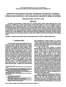
When the network is being trained, the network itself reaches a compromise between the resolution (the precision) and the depth of its memory in order to carry out the required tasks. RNNs showed a higher capacity of modeling than MLPs, obtaining more accurate results with, in many cases, fewer parameters. In the majority of the cases the training is achieved with the help of the Backpropagation Through Time off-line algorithm. The use of Backpropagation Through Time is caused by the inability of backpropagation feed-forward algorithm [3] to be implemented directly into recurrent neural network, because the backpropagation pass presupposes that the connections between the neurons induce a cycle-free oerdering. Backpropagation algorithm modifications for recurrent neural networks is named Backpropagation Through Time. In this algorithm, considering a time-series of length l, the central idea of BPTT algorithm is to unfold the original recurrent neural networks in time so as to obtain a feedforward network with l layers, which in turn makes it possible to implement the learning method by backpropagation through time to diminish gradient error. BPTT unfold the network in time by stacking identical copies of the RNNs, and duplicating connections within the network to obtain connections between subsequent copies. The weights between successive layers must remain identical in order to be able to show up in the original recurrent neural network. In practice, it amounts to cumulating the changes of the weights for all the copies of a particular connection and adding the sum of the changes to all these copies after each learning iteration. Figure 1. shows a very simple recurrent neural network architecture, where there are only two units: input unit and output unit, and there is only one layer on this recurrent neural network architecture. Arrow lines show interconnections between nodes on the neural network. It can be seen that there are a few additional connections if it is compared with a standard feed-forward network, namely connections from output unit to input unit, and connections from input unit and output unit to the unit itself. Figure 2. shows the shape of actual recurrent neural network architecture that will be used on recurrent neural network implementation as base learner from boosting method, where the nodes appointed by arrow lines that are marked by x1(t) are the input neurons, and the output neurons are neurons that generated an arrow lines from itself and is marked by y1(t). On the actual implementation, a single input neuron input

Figure 1. A simple recurrent neural network

Figure 2. Recurrent neural network unfolded in time

and a single linier output neuron will be used, along with an additional single bias node and hidden nodes that the exact amount of them is inputted by user. Activation function used for this recurrent neural network is sigmoid symmetric activation function or mathematically, function tanh that having a output value ranged between -1 and 1. Considering the application of BPTT for the training of recurrent neural networks between time t1 and tl. fi is the transfer function or activation function of neuron i, si(t) its output at time t, and wij its connection being from neuron j. A value provided to the neuron at time t coming from outside is noted xi(t). Backpropagation through time algorithm supposes an evolution of neurons of recurrent neural networks given by the following equations: (1) s i(t) = f(net i(t − 1)) + x i(t), i = 1,..., N

net i(t − 1) = ∑ j ∈Prev(i) w ij (t − 1)s j(t − 1)

(2)

a sum function from neuron net i(t − 1) is s j(t − 1) multiplied with associated weight from that neuron, w ij (t − 1) .(t − 1) shows a time counter used dan j value is an index associated with neuron and or weight that are exist within the recurrent neural network. Equation (3) shows the error function used, namely mean quadratic error function. Variable d p (t) shows the target (desired output) from recurrent neural network. Because on the actual implementation input and output neuron using only up to one neuron, so it can be said that the target (desired output) itself is the same as the neural network input on its next iteration, or layer. This principle can only be used on single

step ahead prediction. And its mathematical form is: d p (t) = x i(t + 1) . tl (3) E(t 1 , t l) = 12 ∑t =t 1 ∑ p ∈T(t) (d p (t) − s p (t)) 2 Variable s p (t) is an output neuron from every layer on the network, and variable T(t) shows a set of neurons which have a target/desired output marked by variable d p (t) at the time τ . Weight changing for minimalizing equation (3) using gradient descent:

Δw ij (t 1, t l

− 1

) = −η

∂ E(t 1 , t l) ∂ w ij

(4) E(t , t ) 1 l ∂ tl − 1 = − η∑ τ = t 1 ∂ w ij (τ ) Δw ij (t 1, t l − 1) shows weight changing on a spesific neural network weight (on this example weight ij) from the first layer, onto next layers, until the output layer is reached. η is learning rate or called alpha value, and w ij (τ ) is the duplication of weight wij of the original recurrent neural network, for the time t = τ . ∂ E(t 1 ,t l) ∂ E(t 1,t l) ∂ net i(τ ) = ∂ w ij (τ ) ∂ net i(τ ) ∂ w ij (τ )

(5)

The equations of BPTT algorithm are finally obtained: • For the output layer: ∂ E(t 1 ,t l) = [s i(t l) − d i(t l)] f i' (net i(τ ) ∂ net i(τ )

for i ∈ T( τ + 1) , else: ∂ E(t 1 ,t l) =0 ∂ net i(τ )

(6)

• For the hidden layer: ⎡ [s i(t l) − d i(t l)] + ⎤ ∂ E(t 1 ,t l) ⎢ ⎥ f ' (net i(τ ) = ∂ E(t 1,t l) w ji (τ + 1) ⎥ i ∂ net i(τ ) ⎢ ∑ ⎢⎣ j∈ Foll(i) ∂ net j(τ + 1) ⎥⎦

for i ∈ T( τ + 1) , else: ∂ E(t 1 ,t l) = ∂ net i(τ )

∑

j ∈ Foll(i)

∂ E(t 1,t l) w ji(τ + 1) f i' (net i(τ ) ∂ net j(τ + 1)

(7)

III. BOOSTING METHOD ON RECURRENT NEURAL NETWORKBACKPROPAGATION THROUGH TIME Boosting is a general method for improving the accuracy of any given learning algorithm [4]. It produces a final solution by

combining or choosing rough and moderately inaccurate decisions offered by different base learners. In boosting, the training set used for each base learner is produced (weighted) based on the performance of the earlier base learner(s) in the series. Therefore, samples incorrectly learned by previous base learner in the series are more emphasized than the correctly learned ones. Boosting had solved many of the practical difficulties of the earlier boosting algorithms. The boosting algorithm first received a training set, {(xq,yq); q = 1,...,Q} as inputs where xq is an example in space X, and yq is a class label in set Y associated with xq. Boosting repeatedly calls a weak (base) learning algorithm in a series of rounds n = 1,...,N. In each round n, the algorithm assigns a distribution or a set of weights over the training set. The weight of training example q during round n is denoted as Dn(q). The weak learner can use Dn(q) on the training examples. Alternatively, the training inputs can be sampled according to Dn(q), and these resampled inputs can be used to train the weak learner. Initially, all the weights are equally set, and the weights of incorrectly classified examples are increased on each repetition so that the learner is forced to focus on the harder examples in the training set. The weak learner has to compute a hypothesis, hn: X → Y with respect to Dn(q). Once hypothesis hn is calculated, AdaBoost uses a parameter α n = (1 − ε n ) / ε n which is a is the pseudo-loss measure of confidence in the predictor. calculated from a loss function Ln(q). Then, update Dn(q) for the next boosting iteration with an equation: Dn+1(q) = Dn(q) α n (1 − L n ( q )) / Z n where Zn is a normalization constant chosen such as Dn+1 is a distribution. At the end of each boosting iteration, the weights of examples misclassified by hn are increased, and the weights of correctly classified examples are decreased, hence the algorithm is forced to focus on “hard” examples. Finally, hypothesis generated by each weak learner will be formed into a final hypothesis, which is the hypothesis with the lowest error value (NMSE value). The modifications to the AdaBoost algorithm were proposed to suit time-series prediction problem. Generally, the use of boosting in prediction is harder than classification. Classifier map the inputs with several classes, while predictor calculate the expected values that are associated with the given inputs; the outputs are neither correct or incorrect (in contrast to classification problem). Rather, performance of a predictor is measured by the prediction error. This leads to the proposed modifications of the AdaBoost algorithm so that it is applicable to real-valued prediction tasks. Implementation steps of modificated boosting algorithm for time-series forecasting can be described as: 1.

Initialize the weights for the examples: D1(q) = 1/Q, (8) where Q is the number of training example. Set the boosting iteration counter on 0: n = 0.

2.

Iterate (a) Change the value of n = n+1. Learn with BPTT a RNN hn, using training samples obtained from the original training set that having a same size as the original training set. Training samples were obtained using sampling with replacement method from the original training set with respect to probabilies associated with each examples from original training set. On this algorithm, the probability associated with each training set example was following Dn(q) value that symbolizing the weight of example q on boosting iteration n. This method is known as boosting with resampling. Calculate NMSE test value obtained from hypothesis generated, then save this calculated NMSE test value, and hypotehesis generated. (b) Update the weights of the examples: (i) Compute Ln(q) for each q = 1,...,Q according to the loss function used: (n) linear (9) L n ( q ) = y q ( xq ) − yq / Sn , squared

Ln

eksponenti al

Ln

2

(10)

( q ) = 1 − exp( − y (qn ) ( x q ) − y q / S n ) ,

(11)

(n)

( q ) = y q ( xq ) − yq / S n2 ,

with S n = sup y ( n ) ( x q ) − y q ; ; q

(12)

q

(ii) Compute Q

εn = ∑ p n ( q ) L n ( q )

(13)

q =1

and α n = (1 − ε n ) / ε n; (iii) The weights of the examples become: 1 + k . p n +1 ( q ) D n +1 ( q ) = Q+k with D ( q ) α n( L n ( q ) − 1) p n +1 ( q ) = n Zn where Zn is a normalizing constant.

(14) (15)

(16)

Until all of the stopping criterion of boosting iteration fulfilled. Variable N denotes the last value of n; 3.

Choose RNN-BPTT that having, within itself, neural network weights that having the smallest error value on test set. di dalamnya memiliki error terkecil pada test set. This aims for boosting having the best generalization for unknown data (test set).

The boosting algorithm used should comply with the restrictions imposed by the general context of application. In this case, it must be able to work well when a limited amount of data is available and accepts RNNs as regressors. The generic algorithm on [5] is followed and had to decide which loss function to use for the regressors, how to update the distribution on the training set and how to form final hypothesis. Updating distribution or training set weights for

this introduced algorithm follows [6], but before they are used for the next regressor, this weights will be transformed using linier transformation in order to prevent the RNNs from simply ignoring the easier examples. Then, resampling method with training example replacement based on the updated distribution (sampling with replacement) [7] will be used. Stopping criterion used for stopping boosting iteration, is the maximum value of N (maximum of 50). The decision to use training sample obtained from the data of training set for the development of each regressor makes it possible to observe the condition according to which the algorithm must be able to treat time series made up of a limited number of data. Modifications of weights Dn(q) using linier transformation make it possible to give more importance to the difficult example without ignoring the easier example, like which is in standard boosting method that does not use linier transformation for weights used on the next boosting iteration, or next regressor learning process. Parameter k makes it possible to regulate this taking into account; when k=0, the difficult examples have the same weights as others. IV. EXPERIMENTAL RESULTS AND ANALYSIS Experiment is done on a Personal Computer with Intel(R) Core(TM)2 Duo CPU E8600 @ 2.4GHz (2 CPUs) processor, 2048 MB RAM memory. Operating system used is Windows XP Professional Version 2002 SP2. Programming languange used for this method implementation is Matlab 7.0.1. Experiment will only be done on the application of new boosting method with RNN-BPTT as its base learner. The aim of this experiment is to prove the superiority of boosting method over the standard RNN-BPTT algorithm (this superiority can be seen over the diminished value of NMSE test), and observation of variable k, which is used for tuning the boosting influence on available example. Experiment will be done on three datasets, Sunspot dataset, MGS17 dataset, and MGS30 dataset. For the sunspot dataset the amount of hidden unit parameter on RNN-BPTT is 1, and 3 on MGS dataset (MGS17 and MGS30). Parameter alpha will TABLE I MEAN NMSE VALUE COMPARISON BETWEEN RNN-BPTT ALGORITHM AND BOOSTING METHOD ON SUNSPOT DATASET Mean NMSE Reduction of Mean NMSE values values (%) RNN-BPTT

0.32062

0

Boosting linier,20

0.23428

26.92907492

Boosting linier,50

0.24596

23.28613312

Boosting linier,120

0.2476

22.77462417

Boosting squared,20

0.24864

22.45025264

Boosting squared,50

0.24948

22.18826025

Boosting squared,120

0.24932

22.23816356

Boosting exponential,20*

0.22938

28.45736386

Boosting exponential,50

0.24612

23.2362298


0.26818

16.35581062

obtained using the best result from all of the experimental result on boosting method obtained on the combination of linier loss function and variable k = 20. Reduction between the best result of RNN-BPTT and boosting method is 24.51%.

Figure 3. Mean NMSE values variation from some values of variable k parameter at one loss function on Sunspot dataset

be set to 0.06 for all datasets. This number (for each of the hidden unit parameter and alpha value are obtained through the experiment done on RNN-BPTT optimalization test independently). On the boosting method experiment, the two additional test parameter used are the combined parameter of loss function (linier, squared and exponential) and variable k (20, 50 and 120 for Sunspot dataset or 20, 150 and 300 for MGS datasets). So there is nine mini scenarios used for boosting method experiment. The number of experiments done for Sunspot dataset are five for each of the mini scenario, and for MackeyGlass datasets are three for each of the mini scenario. A. Boosting Method Experiment on Sunspot Dataset Sunspot data set is a natural dataset that contains the yearly number of dark spots on the sun from 1700 to1979. Training set used from this time-series dataset are data from years 1700 to 1920 (221 data), and test set used from this time-series dataset are data from years 1921 to 1955 (35 data). From table I. can be seen that the highest reduction of mean NMSE values from RNN-BPTT algorithm to boosting method is obtained from exponential loss function parameter with variable k = 20. Reduction obtained from this experimentation is 28.45%. From figure 3. it can be seen that along with the increased variable k value on a loss function, then the mean NMSE value is also increasing (it means that the leaning algorithm is performing worse). There is an exceptional loss function which if variable k value was to be increased, the performance of the learning algorithm is performing better, which is squared loss function. On this loss function, the alteration of variabel k values from 50 to 120 makes the boosting method performs better. With the squared loss function as an exception, other loss functions tend to show a same disposition for alteration of variable k associated with it. From figure 4. it can be seen that test set prediction from Sunspot dataset using boosting method is satisfying if it was to be compared with result obtained from RNN-BPTT algorithm. Using the boosting method, the shape and the bounds from the test set prediction plotting is becoming more like the plotting from the actual test set. Plotting showed on figure 4 is

B. Boosting Method Experiment on MGS17 Dataset Mackey-Glass dataset, or Mackey-Glass benchmark is a dataset generated by this following nonlinier differential equation: 0 .2 x (t − θ ) dx (17) = − 0 .1 x (t ) + dt 1 + x 10 ( t − θ ) This time-series dataset had a chaotic behaviour for the values of θ > 16,8. Because of this behaviour, Mackey-Glass time-series is usually used for the capability evaluation of forecasting methods. On MGS17 dataset, variable θ value used is 17. But for Mackey-Glass dataset, θ = 17 (MG17) or θ = 30 (MG30), the training set used from this time-series data is obtained from the first 500 data, and the next 100 data are used as the test set. From table II. it can be seen that the highest reduction of mean NMSE values from RNN-BPTT algorithm to boosting method is obtained from squared loss function parameter with variable k = 20. Reduction obtained from this experimentation is 84%. If it was compared with experimental results obtained from Sunspot dataset, boosting method proved to be more effective if used on MGS17 dataset with performance improvement around 55 to 60%. From figure 5. it can be seen that along with the increased variable k value on a loss function, then the mean NMSE value is also increasing (it means that the leaning algorithm is performing worse). There is an exceptional loss function which if variable k value was to be increased, the performance of the learning algorithm is performing better, which is exponential loss function. On this loss function, the augmentation of variabel k values makes the boosting method performs better. With the exponential loss function as an exception, other loss functions tend to show a same disposition for alteration of variable k associated with it. TABLE II MEAN NMSE VALUE COMPARISON BETWEEN RNN-BPTT ALGORITHM AND BOOSTING METHOD ON MGS17 DATASET Mean Reduction of Mean NMSE NMSE values (%) RNN-BPTT

0.1254

0

Boosting linier,20

0.02193

82.50930356

Boosting linier,150

0.022467

82.08399787

Boosting linier,300

0.02273

81.87134503

Boosting squared,20*

0.02

84.05103668


0.0214

82.93460925


0.02483

80.19670388


0.0235

81.2599681


0.021

83.25358852


0.020267

83.83838384

Figure 4. Comparison of test set plotting on the actual dataset with test set forecasting using RNN-BPTT and boosting method on Sunspot dataset

Figure 5. Mean NMSE values variation from some values of variable k parameter at one same loss function on MGS17 dataset.

From figure 6. it can be seen that test set prediction from MGS17 dataset using boosting method is satisfying if it was to be compared with result obtained from RNN-BPTT algorithm. Using the boosting method, the shape and the bounds from the test set prediction plotting is becoming more like the plotting from the actual test set. Plotting showed on figure 6 is obtained using the best result from all of the experimental result on boosting method obtained on the combination of exponential loss function and variable k = 300. Reduction percent between the best result of RNN-BPTT and boosting method is 76.72%. C. Boosting Method Experiment on MGS30 Dataset On MGS30 dataset, equation used to generate this dataset is the same used by MGS17 dataset: 0 .2 x (t − θ ) dx (18) = − 0 .1 x (t ) + dt 1 + x 10 ( t − θ ) with variable θ value used is 30.

Figure 6. Comparison of test set plotting on the actual dataset with test set forecasting using RNN-BPTT and boosting method on MGS17 dataset

On this boosting method experiment of MGS30 dataset, experimental method and the testing step used is a little different with the first two experiment. This because the perfomance of RNN-BPTT algorithm can be said to be experiencing some constraints and can be said to be failed on forecasting the test set of MGS30 dataset. This has an impact on the high NMSE values (it means that RNN-BPTT is performing poorly) on forecasting the test set of MGS30 dataset. On the earlier experiment, it is known that for the RNN-BPTT algorithm to perform at least significantly better, the size of the training set and test set from the dataset used must be increased too (but this method won’t be discussed further). Because of it, on this experiment there will be no comparison between NMSE values of RNN-BPTT algorithm and boosting method. From table III. it can be seen that the lowest mean NMSE values from the boosting method variation is obtained from the combination between squared loss function parameter, with variable k = 20. As said before, there will be no comparison between RNN-BPTT algorithm and boosting method, because of the poor performance of RNN-BPTT algorithm on test set forecasting from MGS30 dataset. If it is truly want to be compared with, the NMSE value reduction from RNN-BPTT to boosting method can achieve values between 95 to 99%. This is the best result obtained between the three experiment done for boosting method test. From figure 7. it can be seen that along with the increased variable k value on a loss function, then the mean NMSE value is also increasing (it means that the leaning algorithm is performing worse). There is an exceptional loss function which if variable k value was to be increased, the performance of the learning algorithm is performing better, which is exponential loss function. On this loss function, the alteration of variabel k values from 20 to 150 makes the boosting method performs better. With the squared loss function as an exception, other

TABLE III MEAN NMSE VALUE COMPARISON BETWEEN RNN-BPTT ALGORITHM AND BOOSTING METHOD ON MGS30 DATASET Mean NMSE value

Figure 7. Mean NMSE values variation from some values of variable k parameter at one same loss function on MGS30 dataset.

Boosting linier,20

0.012533333

Boosting linier,150

0.012866667

Boosting linier,300

0.012966667

Boosting squared,20*

0.012066667


0.012566667


0.013166667


0.0126


0.012466667


0.012766667

algorithm, this experiment also proved that boosting method is superior from standard RNN-BPTT algorithm through all of the testing scenario. V. CONCLUSION

Figure 8. Comparison of test set plotting on the actual dataset with test set forecasting using RNN-BPTT and boosting method on MGS30 dataset

loss functions tend to show a same disposition for alteration of variable k associated with it. From figure 8. it can be seen that test set prediction from MGS30 dataset using boosting method is very satisfying if it was to be compared with result obtained from RNN-BPTT algorithm. Using the boosting method, the shape and the bounds from the test set prediction plotting is becoming more like the plotting from the actual test set. Plotting showed on figure 8 is obtained using the best result from all of the experimental result on boosting method obtained on the combination of square loss function and variable k = 20. From this three experiments done on boosting method to observe changes of mean NMSE values that were affected by the changes of variable k values, it can be seen that the changes from the mean NMSE values are not independently caused only by alteration of variable k values or only alteration of loss function used on boosting method.. Anomaly from variable k behaviour is often found on exponential loss function. In addition to shows the most performance increase that is marked by greatly dimishing NMSE values from RNN-BPTT

After experimenting and analyzing the software that has been made, then the conclusion can be drawn as follows: • Recurrent neural network using backpropagation through time learning algorithm can be used on the single-step ahead time-series forecasting with good results, on some spesific time-series dataset, namely Sunspot dataset, and MGS17 dataset. • To be applied in time-series forecasting, single-step ahead prediction maximally, RNN-BPTT parameters must be determined first. Optimal input parameters for forecasting Sunspot dataset using RNN-BPTT is 1 hidden unit and 0.06 for the value of alpha. For Mackey-Glass dataset, the optimal input parameter is 3 hidden units and 0.06 for the value of alpha. • Boosting method is proved to be better than the standard RNN-BPTT algorithm, marked by the performance increase on all of the testing scenario. For Sunspot dataset, the performance improvement can reach to 25 to 30%, better on the MGS17 dataset with improvement between 80 to 85%, and is the best at the MGS30 dataset with performance improvement obtained is almost 100%. • New variable introduced into boosting method for tuning the boosting influence for time-series forecasting, namely variable k, has been proved to be used for tuning the boosting influence for the forecasting results from timeseries data single-step ahead, where on the majority observation from the experimental results show that the smaller values of variable k yield a smaller NMSE value too. Of course this conclusion is not depending only from the choice of variable k, but also from the choice of loss funtion used. REFERENCES [1] A. Alexandre Trindade, Chris Chatfield, Boca Raton, FL: Time Series Forecasting, Chapman and Hall/CRC, 2000.

[2] R. Bone, M.Assaad, H.Cardot: A New Boosting Algorithm for Improved time-series forecasting with Recurrent Neural Networks, Information Fusion 9, pp.41-55, 2008. [3] http://www.learnartificialneuralnetworks.com/backpropaga tion.html, 11 Juni 2009 [4] Y.Freund, R.E. Schapire: A Short Introduction to Boosting, Journal of Japanese Society for Artificial Intelligence 14(5):771-780, September 1999. [5] Y.Freund, R.E. Schapire, A decision-theoretic generalization of online learning and an application to boosting, Journal of Computer and System Sciences 55(1) (1997) 119-139. [6] H.Drucker, Improving Regressor using Boosting Techniques, in: Proceedings of the Fourteenth International Conference on Machine Learning, 1997,pp. 107-115. [7] Schwenk.H,Bengio.Y: Boosting Neural Networks, in: Neural Computation,pp.1869-1887, vol.2, 2000.