IMPROVING PERFORMANCE OF RECURRENT NEURAL NETWORK ...

Under review as a conference paper at ICLR 2016

I MPROVING

PERFORMANCE OF RECURRENT NEURAL NETWORK WITH RELU NONLINEARITY

arXiv:1511.03771v1 [cs.NE] 12 Nov 2015

Sachin S. Talathi & Aniket Vartak Qualcomm Research San Diego, CA 92121, USA {stalathi,avartak}@qti.qualcomm.com

A BSTRACT In recent years significant progress has been made in successfully training recurrent neural networks (RNNs) on sequence learning problems involving long range temporal dependencies. The progress has been made on three fronts: (a) Algorithmic improvements involving sophisticated optimization techniques, (b) network design involving complex hidden layer nodes and specialized recurrent layer connections and (c) weight initialization methods. In this paper, we focus on recently proposed weight initialization with identity matrix for the recurrent weights in a RNN. This initialization is specifically proposed for hidden nodes with Rectified Linear Unit (ReLU) non linearity. We offer a simple dynamical systems perspective on weight initialization process, which allows us to propose a modified weight initialization strategy. We show that this initialization technique leads to successfully training RNNs composed of ReLUs. We demonstrate that our proposal produces comparable or better solution for three toy problems involving long range temporal structure: the addition problem, the multiplication problem and the MNIST classification problem using sequence of pixels. In addition, we present results for a benchmark action recognition problem.

1

I NTRODUCTION

Recurrent neural networks (RNNs) are neural networks with cyclical connections between the hidden nodes. These cyclical connections offer RNNs the ability to encode memory and as such these networks, if successfully trained, are suitable for sequence learning applications. Traditionally, training RNNs using stochastic gradient descent methods such as back-propagation through time (BPTT) (Rumelhart et al., 1986) have been riddled with difficulty. Early attempts suffered from the so-called vanishing gradient or exploding gradient problems resulting in difficulties to learn longrange temporal dependencies (Hochreiter et al., 2001). Several methods have been proposed to overcome the difficulty in training RNNs. These methods broadly fall into three categories: (i) Algorithmic improvements involving sophisticated optimization techniques. The Hessian-Free (HF) optimization method (Martens, 2010; Martens & Sutskever, 2011) for training RNNs falls under this category. HF method works by taking large steps in the weight space in directions of low gradient and curvature. As noted by the authors, it is the ability of HF to identify and pursue these directions, which allow HF to fully optimize deep neural networks, such as the RNNs unfolded in time. (ii) Network design, the most successful technique to date under this category is the Long Short Term Memory (LSTM) RNN (Hochreiter & Schmidhuber, 1997). The LSTM is a standard RNN in which the monotonic nonlinearity such as the tanh or sigmoid is replaced with a memory unit that can efficiently store continuous values and transmit information over a long temporal range. Each memory unit in the LSTM has fixed linear dynamics with a feedback loop of weight one. As a result the error signal neither decays nor explodes as it back propagates through the memory unit. LSTM RNNs and variants thereof (Cho et al., 2014) have produced impressive results on several sequence learning tasks including handwritting recognition (Graves, 2013), speech recognition (Graves & Jaitly, 2014), machine translation (Cho et al., 2014; Bahdanau et al., 2014), image captioning (Kiros et al., 2014), predicting output of simple computer programs (Zaremba & Sutskever, 2014) and action recognition from video clips (Ng Yue-Hui et al., 1

Under review as a conference paper at ICLR 2016

2015). More recently, a modification to the standard RNN architecture, the clockwork RNN (CWRNN) has been proposed (Koutn´ık et al., 2014). The long range dependency problem of vanishing and exploding gradients in the standard RNN is solved in CW-RNN by dividing the hidden layer of the CW-RNN into separate modules, each running at different clock speeds. This allows CW-RNNs to efficiently learn different time scales inherent in complex-signals. (iii) Weight initialization, more recently Quoc et al, (Quoc et al., 2015) proposed a simpler solution to the long-range dependence problem with RNNs composed of rectified linear units (RELU)s. The authors proposed to use the Identity matrix to initialize the recurrent weight matrix.They call the resulting RNN, Identity-RNN (IRNN). The basic idea underlying IRNN is that in the absence of any input, a RNN composed of RELUs and initialized with identity weight matrix just stays the same indefinitely. Experimental results with IRNN on several benchmark problems with long-range temporal structure are comparable to the those produced by LSTM RNNs (Quoc et al., 2015). In this paper, we investigate the significance of identity weight initialization in IRNNs from a dynamical systems perspective. We demonstrate that in absence of any input and with identity weight initialization the hidden nodes exhibit neutrally stable fixed point dynamics. While this observation produces the effect that the hidden node dynamics stays the same indefinitely in absence of any input, the node dynamics is also extremely sensitive to input perturbations. We hypothesize that this sensitivity of hidden node dynamics to input may influence the success of RNN for sequence learning tasks. Motivated by this hypothesis we propose a new weight initialization matrix, the normalized-positive definite weight matrix for RNNs comprised of RELU hidden units. The resulting RNN is refered to as the np-RNN. We show that on several of the tasks investigated by (Quoc et al., 2015), np-RNN performs better than IRNN or the corresponding scaled version of the IRNN, the iRNN, where the recurrent weight matrix is initialized to 0.01I. The paper is organized as follows: In Section 2, we describe the simple RNN (sRNN) model and explain how the identity weight matrix initialization for hidden layer weights provide initial conditions to alleviate the long range problem in training sRNN. We then offer a dynamical systems perspective on the identity matrix weight initialization and present our proposal for weight initialization of hidden layer weight matrix to construct the np-RNN. In Section 3, we present an overview of the experiments to evaluate the performance of np-RNN, followed by results from our experiments on benchmark datasets in Section 4. The conclusion is presented in Section 5.

2

DYNAMICAL SYSTEMS PERSPECTIVE ON RNN S

yt Wyh

Whh

ht Whx xt

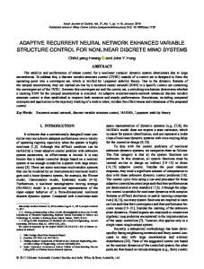
Figure 1: Schematic diagram of a simple RNN network

In Figure 1 we show the schematic of a sRNN. The sRNN consists of an input layer, a hidden layer with recurrent connections and an output layer. Given an input sequence X = {x0 , x1 , x2 · · · xT }, the sRNN will take the input xt ∈ RN and generate the prediction yt ∈ RC for the output sequence Z = {z0 , z1 , z2 · · · zT }, where zt ∈ RC . In between the input and the output there is a hidden layer 0 with M units, which store information on the previous values (t < t) of the input sequence. More precisely, the sRNN takes X as input and generates an estimate Y of the output Z by iterating the 2

Under review as a conference paper at ICLR 2016

equations st ht ot yt

= = = =

Whx xt + Whh ht−1 + bh f (st ) Wyh ht + by g(ot )

(1) (2) (3) (4)

where Whx , Whh and Wyh are the weight matrices, bh and by are the biases, st ∈ RM and ot ∈ RC are inputs to the hidden layer and the output layer respectively and f and g are functions. For the purpose of this paper, f is a ReLU and depending on the benchmark under investigations; g is a linear function or a softmax function. In addition; all hidden layer nodes are assumed to be initialized to a fixed bias bi such that at t=0 h0 = bi . Unless otherwise stated, for all experiments we set bi = P 0. The objective function, O(θ) for sRNN with a single training pair (x,y) is defined as O(θ) = the set of parameters (weights and biases) in the t Lt (z, y(θ)), where θ represents

(zt − yt )2 and for multi-class classification problems, sRNN. For regression problems, L = t P Lt = − j ztj log(ytj ). The IRNN model proposed by (Quoc et al., 2015) is a special case of sRNN with the following modifications: (i) the nonlinearity f is RELU and (ii) the hidden layer weights Whh are initialized with identity matrix and the bias terms are set to zero. In order to better understand how these modifications may enable RNN to overcome some of the long range problems, let us look at the gradient equation in the BPTT algorithm (Pascanu et al., 2013): X ∂Lt ∂C = (5) ∂θ ∂θ t≤T

=

X ∂Lt ∂hT ∂ + ht ∂hT ∂ht ∂θ

(6)

∂hT ∂hT −1 ∂ht+1 ··· ∂hT −1 ∂hT −2 ∂ht

(7)

t≤T

where, ∂hT ∂ht

=

t+1 Each Jacobian ∂h ∂ht is a product of two matrices: (a) the recurrent weight matrix Whh and (b) diagonal matrix composed of the derivative of non-linearity, f , associated with the hidden nodes. In absence of any input, i.e., xt = 0, and with the choice of initial conditions for IRNN,the 2Norm of each Jacobian in Equation 7 is identically one and the error gradients do not grow or decay exponential over time.

In order to understand what the design of IRNNs means from a dynamical systems perspective, let us consider a simple example of sRNN with two hidden nodes with ReLU nonlinearity. We again assume that the sRNN receives zero input and all the biases are set to zero. We further assume that the recurrent weight matrix, Whh , is positive definite. The dynamics of hidden nodes is then given by the following equation: ht

= Whh ht−1 if ht−1 > 0 = 0 ohterwise

(8)

In Figure 2a-d, we show the schematic diagram of the phase-space of the hidden node dynamical system in Equation 8, dependent on the eigenvalues, λ, of the recurrent weight matrix (Strogatz, 2014). The IRNN model corresponds to the case shown in Figure 2a. In absence of any perturbations, every choice of initial conditions for the hidden nodes represents a fixed point that is neutrally stable. As a result, the evolution of the hidden node dynamics is strongly dependent on the input perturbations. The dynamics in 2b, corresponds to the case when all eigenvalues are less than 1. In this case, the hidden node dynamical system has a single stable fixed point at the origin. In absence of any input the the hidden nodes will evolve to zero. Increasingly stronger input perturbations are required to prevent the hidden node dynamics from evolving to origin as the hidden nodes evolve closer to the stable fixed point. 3

Under review as a conference paper at ICLR 2016

a

b

h1 0 1

=1 =1

h1 0 1

10 s into one of the 101 action classes. The benchmark contains a total of 13320 video clips divided into 25 groups. Each group contain video clips from all 101 action classes. Video clips of a given action in a given group share some commonalities. Usually the performance of a given classifier on this data set is evaluated using three splits of the training/testing data. For our experiments we report results for the split one, with training data made up of video clips from groups 8-24 and the test data made up of videos derived from groups 1-7. 5

Under review as a conference paper at ICLR 2016

4 4.1

R ESULTS A DDITION P ROBLEM

As suggested in (Quoc et al., 2015), a basic baseline solution would be to always predict 1 as the output regardless of the inputs. This will produce a Mean Squared Error (MSE) of approximately 0.166. To solve this problem the recurrent net has to remember the two relevant numbers and their sum while ignoring the irrelevant numbers. The task gets difficult with increasing length T of the sequence.

Correctly predicted test examples

In order to evaluate the RNN networks (iRNN,IRNN,np-RNN,gRNN) we generate 100,000 training examples and 10,000 test examples. For all the reported results, we trained the network using SGDBPTT optimization. The learning rate was fixed at 0.001 and the gradient clip parameter was set to 10. The batchsize was set to 1 and all the networks were trained for 10 epochs. Following from (Quoc et al., 2015), we began by evaluating the performance of RNNs on the addition benchmark for sequences of length T = {150, 200, 300, 400}.

Figure 3: Bar chart of correctly predicted test examples for the addition problem The results are summarized in Figure 3. We plot the total number of correctly classified sequences in the test data, defined as the sequences for which the absolute prediction error is less than 0.04 (Martens & Sutskever, 2011). For sequences up to T = 300, our results for gRNN and IRNN match those obtained by (Quoc et al., 2015). We also note that the np-RNN performs at par or better than the other RNNs for T 90 % for all sequences investigated. 4.3

MNIST CLASSIFICATION WITH SEQUENTIAL PRESENTATION OF PIXELS

This is another challenging toy problem where the goal is to classify MNIST digits (Lecun et al.) when the 784 pixels are presented sequentially to the RNN. The network is asked to predict the digit after all the 784 pixels are presented to the RNN serially one pixel at a time. We began by first attempting to reproduce the findings from (Quoc et al., 2015). However using the SGD-BPTT optimization, we were unable to train IRNN on MNIST using the set of parameters reported in (Quoc et al., 2015). Using RMSprop (Tieleman & Hinton), however, we were successful in training IRNN with learning parameter of 10−6 . The np-RNN was trained using SGD-BPTT optimization with cooling. We trained both IRNN and np-RNN network for 100 epochs with batch size of 16, corresponding to about 375000 iterations. The np-RNN was trained for 33 epochs with initial learning rate of 10−4 , followed by training for another 33 epochs with learning rate cooled by factor of 10 and then again trained unto 100 epochs by cooling learning rate by another factor of 10. In Figure 5, we plot the evolution of the cost function on the test batch as a function of the number of epochs. The resulting accuracy is reported in Table 2. We note that while the IRNN produces accuracy of about 83 %, the np-RNN produces an accuracy of about 92 %, which is inline with the results reported by (Quoc et al., 2015). The accuracy grows to 96.8% on training the np-RNN for 500 epochs,which corresponds to 937500 epochs, while for IRNN trained with the given parameters, the accuracy grows to about 93%. Based on our findings on the performance of IRNN and np-RNN on the action recognition benchmark (see Section 4.4) and our inability to reproduce the results reported in (Quoc et al., 2015), we conclude that IRNN is extremely sensitive to the choice of the training protocol and the hyper parameters of the network. On the other hand, the observation that np-RNN performs as well as published results for this toy problem is encouraging. 4.4

ACTION RECOGNITION BENCHMARK

We also benchmarked IRNN, np-RNN and the LSTMs on the UCF-101 action recognition dataset (Soomro et al., 2012). We followed the approach proposed in (Ng Yue-Hui et al., 2015) and trained the RNNs on the sequence of features generated by passing the sequence of video frames through a 7

Under review as a conference paper at ICLR 2016

Figure 5: The loss function on the test data plotted as function of the number of epochs. The dotted lines correspond to the times when the learning rate was cooled by a factor of 10. Note the high variability in the loss function for np-RNN in the first phase of learning is because of large choice for initial learning rate relative to those used in training the IRNN.

RNN Type

Training Method

IRNN np-RNN

RMSProp SGD-BPTT

Accuracy 100 epochs 83 % 92 %

Accuracy 500 epochs 93 % 96.8 %

Table 2: Performance on MNIST digit classification

pre-trained Convolutional Neural Network (CNN). Motivated by the recent findings of (Jain et al., 2015), we use a CNN trained on 15000 Imagenet object categories as the feature generator. The CNN architecture was modeled after the Googlenet-CNN (Szegedy et al., 2014) and the features were extracted from the last fully-connected layer of the Googlenet-CNN. The UCF101 benchmark contains 13,320 video clips, divided into 25 groups. The groups are divided into 3 splits of training and testing for evaluation. As the training data is very small, we did not fine tune the CNN, but rather only focused on training the RNNs using raw features generated by a pretrained feature learner. Furthermore to avoid overfitting, we introduced dropout between the hidden and the output layer of the RNN. Our implementation of LSTM was standard including the forget gate. For all the 3 RNNs, we did a grid search over learning rates l = {10−5 , 5 × 10−5 , 10−4 , 5 × 10−4 , 10−3 , 10−2 } and the dropout parameter d = {0.5, 0.7, 0.9}. The training protocol was: RMSprop for optimization, batchsize of 256, training for a total of 70 epochs, with training for the first 25 epochs with initial learning rate, followed by training for additional 30 epochs with learning rate cooled by factor of 10 and final phase training for additional 15 epochs by cooling the learning rate by another factor of 10. For all our investigations, we used the split one of the training/testing data comprised of video clips from groups 8 through 25 in the training set and video clips from group 1 through 7 in the test set. In order to search over the space of hyperparameters {l, d}, we further split the split one training data into training and validation data set. Data from groups 8 through 24 was used to train all the RNNs and data from group 25 was used for validation. In Table 3 we report the score on the split one test data using RNN with best validation score over the grid search. The scores for np-RNN are closer to LSTM than IRNN and are comparable to the published state-of-the-art for split one of training/test 8

Under review as a conference paper at ICLR 2016

Accuracy

Dropout

c

b

a

0.9

0.7

-5

-4.3 -4

-3.3 -3

-2

-5

-4.3 -4

-3.3 -3

-2

-5

-4.3 -4 -3.3 -3

-2

Learning rate (log scale)

Figure 6: Plot of accuracy on the validation data as a function of the grid search parameters: Learning rate and dropout for (a) IRNN (b)np-RNN and (c) LSTM

RNN Type IRNN np-RNN LSTM

Accuracy validation

Training Method RMSProp (l=10−2 ; d=0.5) RMSProp (l=10−3 ; d=0.5) RMSProp (l=10−3 ; d=0.5)

71 %

Accuracy test 67 %

78.6 %

75.2 %

80.3 %

78.5 %

Table 3: Performance of RNNs on split one of UCF101 benchmark

data for the UCF101 benchmark (Ng Yue-Hui et al., 2015; Jain et al., 2015). Note that while the LSTM produces the best scores for this benchmark, LSTM is five times computational complex relative to the sRNN (Klaus et al., 2015). In Figure 6, we plot the validation scores for the 3 RNNs as function of the grid search parameters. It is clear from the Figure that the performance of IRNN is much strongly dependent on the right choice of hyperparameters, which is not the case for np-RNN or the LSTM.

5

C ONCLUSION

We offer a dynamical systems perspective on the Identity weight initialization for the recurrent weight matrix for RNNs with hidden nodes made up of ReLUs. We hypothesize that the sensitivity of hidden nodes to input perturbations resulting from the Identity weight matrix initialization, may make IRNN sensitive to the choice of hyperparameters for successful training. We offer an alternative weight initialization strategy, the normalized positive-definite weight matrix, that attempts to reduce the sensitivity of the hidden nodes to input perturbations by collapsing the dynamics to a one-dimensional manifold. We compare the performance of IRNN to np-RNN on several toy examples and also one real world action recognition benchmark and demonstrate that np-RNN either performs better or is comparable to IRNN on these benchmarks. ACKNOWLEDGMENTS We acknowledge valuable feedback from our colleagues at Qualcomm Research: Daniel Fontijne and Anthony Sarah. 9

Under review as a conference paper at ICLR 2016

R EFERENCES Bahdanau, D., Cho, K., and Y., Bengio. Neural machine translation by jointly learning to alogn and translate. arXiv:1409.0473, 2014. Cho, K., van Merrienboer, B., Gulcehre, C., Bahdanau, D., Bougares, F., Schwenk, H., and Y., Bengio. Learning phrase representations using rnn encoder-decoder for statistical machine translation. arXiv:1406.1078, 2014. Glorot, X. and Bengio, Y. Understanding the difficulty of training deep feedforward neural networks. In 13th International Conference on Artificial Intelligence and Statistics, 2019. Graves, A. Generating sequences with recurrent neural networks. arXiv:1308.0850, 2013. Graves, A. and Jaitly, N. Towards end-to-end speech recognition with recurrent neural networks. In Proceedings of 31st Internation Conference on Machine Learning, 2014. Hochreiter, S. and Schmidhuber, J. Long short-term memory. Neural Computation, 1997. Hochreiter, S., Bengio, Y., Frasconi, P., and Schmidhuber, J. A field guide to dynamical recurrent network, chapter Gradient flow in recurrent nets. IEEE Press, 2001. Jain, M., van Gemert, J.C., and Snoek, C. The schematic diagram of the work flow for training rnn on ucf-101 benchmark is shown in figure 6. In In IEEE conference on Computer Vision and Pattern Recognition, 2015. Kiros, R., Salakhutdinov, R., and Zemel, R.S. Unifying visual-semantic embeddings with multimodal neural language models. arXiv:1411.2539, 2014. Klaus, G., Srivastava, R.K., Koutnik, J., Steunebrink, B.R., and Schmidheuber, J. Lstm: A search space odyssey. arXiv:1503.04069, 2015. Koutn´ık, J., Greff, K., Gomez, F., and Schmidhuber, J. A clockwork rnn. arXiv:1402L3511, 2014. Lecun, Y., Cortes, C., and Burges, J.C. Mnist handwritten digit database. Martens, J. Deep learning via hessian-free optimization. In In Proceedings of 27th International Conference on Machine Learning, 2010. Martens, J. and Sutskever, I. Learning recurrent neural networks with hessian-free optimization. In In Proceedings of the 28th International Conference on Machine Learning, 2011. Ng Yue-Hui, J., Hausknecht, M., Vijayanarasimhan, S., Vinyals, O., Monga, R., and Toderici, G. Beyond short snippets: Deep networks for video classification. arXiv:1503.08909, 2015. Pascanu, R., Mikolov, T., and Bengio, Y. On the difficulty of training recurrent neural networks. arXiv:1211.5063, 2013. Quoc, V.L., J., Navdeep, and G.E., Hinton. A simple way to initialize recurrent network of rectified linear units. arXiv:1504.00941, 2015. Rumelhart, D., Hinton, G.E., and Williams, R.J. Learning representations by back-propagating error. Nature, 323:533–536, 1986. Soomro, K., Zamir, A.R., and Shah, M. Ucf101: A dataset of 101 human actions classes from videos in the wild. arXiv:1212.0402, 2012. Strogatz, S. Nonlinear Dynamics and Chaos: With Applications to Physics, Biology, Chemistry, and Engineering. Westview Press, second edition, 2014. Sussillo, D. and Abbott, A. arXiv:1412.6558, 2015.

Random walk intialization for training very deep networks.

Szegedy, C., Liu, W., Jia, Y., Sermanet, P., Reed, S., Anguelov, D., Erhan, D., Vanhoucke, V., and Rabinovich, A. Going deeper with convolutions. arXiv:1409.4842, 2014. 10

Under review as a conference paper at ICLR 2016

Tieleman, T. and Hinton, G. Divide the gradient by a running average of its recent magnitude. Lecture 6.5-rmsprop, COURSERA: Neural networks for machine learning. Zaremba, W. and Sutskever, I. Learning to execute. arXiv:1411.4555, 2014.

11