James D. Meernik, Acting Dean of the Robert. B. Toulouse School of ..... band-pass signal of frequency up to 32MHz based on Nyquist principle. Full range on ...
IMPLEMENTATION OF TURBO CODES ON GNU RADIO Mahendra Talasila
Thesis Prepared for the Degree of MASTER OF SCIENCE
UNIVERSITY OF NORTH TEXAS December 2010
APPROVED: Shengli Fu, Major Professor and Graduate Program Coordinator Murali R. Varanasi, Committee Member and Chair of the Department of Electrical Engineering Yan Wan, Committee Member Costas Tsatsoulis, Dean of College of Engineering James D. Meernik, Acting Dean of the Robert B. Toulouse School of Graduate Studies
Talasila, Mahendra. Implementation of turbo codes on GNU radio. Master of Science (Electrical Engineering), December 2010, 67 pp., 34 figures, 2 tables, bibliography, 20 titles. This thesis investigates the design and implementation of turbo codes over the GNU radio. The turbo codes is a class of iterative channel codes which demonstrates strong capability for error correction. A software defined radio (SDR) is a communication system which can implement different modulation schemes and tune to any frequency band by means of software that can control the programmable hardware. SDR utilizes the general purpose computer to perform certain signal processing techniques. We implement a turbo coding system using the Universal Software Radio Peripheral (USRP), a widely used SDR platform from Ettus. Detail configuration and performance comparison are also provided in this research.
Copyright 2010 by Mahendra Talasila
ii
ACKNOWLEDGMENTS First I would like to express my gratitude to Dr. Shengli Fu, for introducing me to the interesting world of GNU radio and encouraging me to pursue my thesis on this topic and for his guidance throughout my stay in the university. Next, I would like to thank Dr. Murali Varanasi and Dr. Yan Wan for their support as committee members of my thesis. I would also like to thank Eric Blossom for providing tutorials to understand the GNU radio programming. I would also like to thank Matthew C. Valenti and Hamid R. Sadjadpour for providing complete details on how to perform turbo coding. Lastly, I am grateful to my family and friends for their support over the years, and especially during the last several months of intense work on this thesis.
iii
CONTENTS LIST OF FIGURES CHAPTER 1.
vii
INTRODUCTION
1
1.1.
Channel Coding
1
1.2.
Software Defined Radio(SDR)
2
1.3.
Realizable SDR
3
CHAPTER 2.
TURBO CODES
5
2.1.
Introduction
5
2.2.
Turbo Encoding
5
2.2.1.
Recursive Encoding
7
2.2.2.
Pseudo Random Interleaving
7
2.3.
Turbo Decoding
2.3.1.
MAP Algorithm
2.3.2.
Max-Log-MAP Algorithm
7 9 11
2.4.
Simulated Results
13
2.5.
Performance Factors
13
2.6.
Selective Serial Concatenation of Turbo Codes
14
2.6.1.
Results
CHAPTER 3.
14
GNU RADIO
16
3.1.
Introduction
16
3.2.
USRP Board
17 iv
3.2.1.
ADC/DAC Converters
17
3.2.2.
Daughter Boards
19
3.2.3.
FPGA
21
3.2.4.
USRP Transmit and Receive paths
23
3.3. 3.3.1. 3.4.
GNU Radio Installation
26
Installing GNU Radio
27
Dial-tone Program
CHAPTER 4.
29
BPSK MODULATION
33
4.1.
Introduction
33
4.2.
BPSK Modulation
34
4.2.1.
System Model
34
4.2.2.
Implementation
35
4.2.3.
Transmission of Data using BPSK
41
4.3.
BPSK Demodulation
43
4.3.1.
System Model
43
4.3.2.
Implementation
43
4.3.3.
Receiver
51
4.4.
Results
CHAPTER 5.
53 TURBO CODES IMPLEMENTATION
56
5.1.
Introduction
56
5.2.
Implementation
56
5.2.1.
Transmitter
56
5.2.2.
Receiver
58
5.3.
Results
CHAPTER 6.
58 DEMO
62 v
6.1.
System without Turbo Coding
62
6.2.
System with Turbo Coding
63
CHAPTER 7.
CONCLUSION AND FUTURE WORK
BIBLIOGRAPHY
65 66
vi
LIST OF FIGURES 1.1
Block diagram of ideal SDR.
2
1.2
Block diagram of realizable SDR.
4
2.1
Example for turbo encoder.
6
2.2
Block diagram of turbo decoder.
8
2.3
Performance of turbo code with r = 12 , k = 5, L = 65536 for various number of decoder iterations.
13
2.4
Selective concatenation scheme.
15
2.5
Performance of selective concatenation scheme.
15
3.1
Block diagram of GNU radio components.
16
3.2
Block diagram of realizable SDR using GNU radio and USRP.
17
3.3
Picture of USRP motherboard.
18
3.4
Picture of USRP with four daughter boards.
18
3.5
USRP block diagram.
19
3.6
RFX400 daughter board.
22
3.7
VERT400 antenna.
22
3.8
Block diagram of digital down converter [10].
23
3.9
Block diagram of digital up converter [10].
24
3.10 USRP transmit and receive signal paths [10]. vii
25
3.11 Flow graph of dial-tone generator.
32
4.1
Constellation diagram of BPSK.
34
4.2
Performance of different PSK schemes.
35
4.3
System model for BPSK modulation.
35
4.4
Complete model for transmission of data using BPSK.
41
4.5
Flow chart for transmission of data using BPSK.
42
4.6
System model for BPSK demodulation.
43
4.7
Complete model for transmission of data using BPSK.
51
4.8
Flow chart for transmission of data using BPSK.
52
4.9
Picture of transmitter sending packets.
54
4.10 Picture of receiver receiving packets.
54
5.1
Block diagram of transmitter using turbo coding.
57
5.2
Block diagram of receiver using turbo coding.
58
5.3
Picture of transmitter sending packets with turbo coding.
59
5.4
Picture of receiver receiving packets with turbo coding.
60
6.1
Block diagram of transmitter to transmit audio file.
63
6.2
Block diagram of receiver to receive audio file.
63
6.3
Block diagram of transmitter to transmit audio file using turbo coding.
64
6.4
Block diagram of receiver to receive audio file using turbo coding.
64
viii
CHAPTER 1 INTRODUCTION 1.1. Channel Coding Channel coding is a technique to ensure that the transmitted signal is recovered at the destination with very low probability of error. The error detection and correction is achieved through adding redundant bits to the transmitted bits. Each redundant bit is obtained from the information bits based on a predetermined rule. The output after channel coding may or may not contain the original information. The codes which include the original information at the output are called systematic codes, while those that do not include the original information are called non systematic codes. The two main categories of channel codes are [20]: (i) Block codes: A block of k message bits is encoded to give a codeword of n bits(n>k).There is a unique codeword of n bits for each sequence of k message bits. Hamming codes and cyclic codes are examples of block codes. (ii) Convolutional codes: The coded sequence depends on the present and the previous information bits.It works on bit streams of arbitrary length. Block codes and convolutional codes can be combined to further increase the performance of the communication system.These concatenated codes are used in satellite and deep space communications [17]. Turbo coding is an iterative soft-decoding algorithm that combines two or more convolutional codes and an inter leaver to produce a block code that can approach Shannon limit. 1
Turbo codes perform better than the convolutional codes but the performance is limited by the decoder latency. More about turbo coding is discussed in chapter 2.
1.2. Software Defined Radio(SDR) A software defined radio (SDR) system is a communication system in which the hardware components are implemented in terms of software on a personal computer. The block diagram of an ideal SDR is shown in Figure 1.1. The idea behind SDR is to implement the modulation and demodulation with software code rather than using a dedicated circuitry. The benefit of using SDR is to handle different types of signals just by loading an appropriate program rather than building circuitry for each of them. Therefore, a single SDR system can be used as one of many radio frequency (RF) transceivers (e.g. , global positioning system (GPS), 802.11, high-definition television (HDTV)) by executing a different block of code.
Figure 1.1.
Block diagram of ideal SDR.
In reality, the ideal SDR in Figure 1.1 is not realizable because: 2
• Antennas are intended to operate within a particular range of frequencies and they cannot operate on entire frequency range. • High speed analog-to-digital converters (ADC) and digital-to-analog converters (DAC) that are used currently are not fast enough to process a large portion of occupied spectrum, and • General purpose computers that are used currently are still inadequate to handle some real-time applications.
1.3. Realizable SDR Currently SDRs are implemented by making use of field programmable gate arrays (FPGA) and super heterodyne mixing stages called RF front ends as shown in Figure 1.2. RF front ends are used to translate the signal from its carrier frequency to an intermediate frequency (IF) or vice versa. This helps in reducing the data rates of ADC/DACs since the ADC/DAC needs to convert the signal over its modulation bandwidth rather than using entire bandwidth. FPGAs can be stationed between the ADC/DAC and the computer in order to reduce the computational burden of the computer by performing computationally expensive signal processing techniques, like digital down/up conversions and decimation/interpolation filtering on, FPGA. The new SDR system is limited to operate in a particular frequency band (due to RF front ends) without any significant affect to flexibility. In this thesis, I implement the turbo coding over SDR. Turbo codes are a class of iterative channel codes which demonstrates the strong capability for error correction. The advantage of SDR is that I can implement different modulation schemes and tune to any frequency band by means of software that can control the programmable hardware. So in this thesis, I am implementing a communication system which makes use of advantages of both turbo codes and SDR. In this report, chapter 3 introduces GNU radio and also explains the installation and usage of GNU radio. Chapter 4 deals with the implementation of binary phase shift keying 3
Figure 1.2.
Block diagram of realizable SDR.
(BPSK) modulation and demodulation. Chapter 5 deals with the implementation of turbo codes and the performance of both systems is compared in this chapter.
4
CHAPTER 2 TURBO CODES 2.1. Introduction Turbo codes are high-performance forward error correcting codes (FEC) with practical decoding algorithm that closely approach the channel capacity proposed by Shannon.In the presence of noise, if one wants to achieve reliable communication with constraints in latency turbo codes are used. Shannon’s equation: Shannon’s equation specifies the maximum rate at which we can transmit information based on the bandwidth, the signal level and the noise level as shown below:
C = Blog2 (1 +
S ) N
where C indicates channel capacity(bits per second) B indicates the bandwidth of the channel(Hz) S indicates the total received signal power(watts) N indicates the total noise(watts) 2.2. Turbo Encoding A turbo encoder is designed by parallel concatenation of two recursive systematic convolutional (RSC) codes separated by an inter leaver. Figure 2.1 shows an example of turbo encoder. Here, the two encoders are
1 2
rate RSC encoders. The upper encoder receives the
data directly where as the lower encoder receives the data after it has been interleaved by a 5
permutation function α. The inter leaver α is in general a pseudo random inter leaver, i.e. it maps bits in position i to position α(i ) according to a prescribed but randomly generated rule. The inter leaver operates in a block wise fashion, interleaving L bits at a time. Since both encoders are systematic, only one of the systematic data needs to be sent. The systematic data of the top encoder is transmitted while that of bottom encoder is not transmitted. The overall code rate of a turbo code composed of two rate can be increased to
1 2
1 2
RSC encoders is 13 . This code rate
by puncturing. The code rate of turbo codes can be increased to
1 2
by
transmitting odd indexed parity bits from upper encoder and even indexed parity bits from lower encoder [1].
Figure 2.1.
Example for turbo encoder.
6
2.2.1. Recursive Encoding In coded systems, performance is dominated by low weight code words. In a good code, low weight outputs are produced with very low probability. An RSC code produces low weight outputs with fairly low probability. The probability that the encoders will have inputs that produce low weight outputs is very low due to presence of the inter leaver. Therefore the combination of these encoders will produce a good code. 2.2.2. Pseudo Random Interleaving In order to achieve the channel capacity proposed by Shannon, we need to develop a random code with large block length. However, decoding the random codes is extremely complex relatively sometimes it may not be possible to decode. Therefore codes must have structure in order to decode them with reasonable complexity. But codes with fixed structure don’t perform like random codes. To solve this problem we need to design a code that appears random but with structure to permit decoding. The pseudo-random inter leaver solves this problem. 2.3. Turbo Decoding An estimate of the information sent can be found by solving a posteriori log-likelihood ratios given by the equations (for further information refer to the reference [1]): � � P mi = 1|y (0) , y (1) , z (2) (1) Λi = log P [mi = 0|y (0) , y (1) , z (2) ] � � P m ˜ i = 1|˜ y (0) , y (2) , z˜(1) (2) ˜ Λ = log i P [m ˜ i = 0|˜ y (0) , y (2) , z˜(1) ] where y (0) is the observed information bits, y (1) is the observed parity bits from encoder on the top, y (2) is the observed parity bits from encoder on the bottom, y˜(0) is the interleaved version of y (0) 7
(2.3.1) (2.3.2)
Λ is the a posteriori log-likelihood ratio (LLR) z is the extrinsic information which is related to LLR by
zi(1) = Λ(1) − yi(0) − zi(2) i
(2.3.3)
˜ (2) − y˜(0) − z˜(1) z˜i(2) = Λ i i i
(2.3.4)
In order to solve the equations from (2.3.1) to (2.3.4), we make use of the structure shown in Figure 2.2. Decoder1 determines solution to equation (2.3.1) and decoder2 determines solution to equation (2.3.2). Each decoder calculates the LLR of the information it receives and sends the extrinsic information to the other decoder and this process is repeated for certain number of iterations. The final estimate of data is obtained by hard limiting the output of one of the decoders [1].
Figure 2.2.
Block diagram of turbo decoder.
8
mi =
1
ifΛ(2) >0 i
0
ifΛ(2) i
(2.3.5)
tmpfile sudo chown root.root tmpfile sudo mv tmpfile /etc/udev/rules.d/10-usrp.rules Now reload the rules of ‘udev’ in order to configure the Ubuntu system to perform certain task when it detects the USRP on the USB by using the command sudo udevadm control −−reload-rules We can check whether USRP is detected by the Ubuntu system by using the command ls -lR /dev/bus/usb | grep usrp If it returns something then the USRP is detected. Now, test whether the GNU radio 28
works with USRP or not, using an example ‘usrp benckmark usb’. To run this example use the commands cd gnuradio-examples/python/usrp ./usrp benchmark usb.py If the program runs properly, then GNU radio and USRP are installed and working properly. Otherwise restart the system and follow the steps shown below: (i) Make a copy from the current ld.so.conf file and save it in a temp folder: cp /etc/ld.so.conf /tmp/ld.so.conf (ii) Add /usr/local/lib path to it : echo /usr/local/lib >> /tmp/ld.so.conf (iii) Add Boost library path to the file: echo /opt/boost 1 37 0/lib >> /tmp/ld.so.conf (iv) Delete the original ld.so.conf file and put the modified file instead: sudo mv /tmp/ld.so.conf /etc/ld.so.conf (v) Do ldconfig: sudo ldconfig After running these commands restart the system and run the example program once again, it must work now.
3.4. Dial-tone Program Let’s go through an example program to understand the usage of the signal processing blocks provided by the GNU radio package in python programming. The dial tone program is often called the ‘Hello world of GNU radio’. This example program includes the generation of dial tone and playing it using audio device available on PC. The dial tone is generated by two sine waves at different frequencies, one on the right channel and the other on the left channel 29
of the audio device. #!/usr/bin/env python from gnuradio import gr from gnuradio import audio
class my top block(gr.top block): def
init (self): gr.top block. init (self) sampling rate = 32000 ampl = 0.1 src0 = gr.sig source f (sampling freq, gr.GR SIN WAVE, 350, ampl) src1 = gr.sig source f (sampling freq, gr.GR SIN WAVE, 440, ampl) dst = audio.sink (sampling f,“”) fg.connect ((src0, 0), (dst, 0)) fg.connect ((src1, 0), (dst, 1))
if
name
== ‘ main ’:
try: my top block().run() except KeyboardInterupt: pass First line in the code ‘#!/usr/bin/env python’ helps us to run the program directly from the command line by giving the program file an executable mode. In order to give the executable mode to the program file, we need to execute the command ‘chmod +x filename’. To use the signal processing blocks that are predetermined in the GNU radio package,
30
we need to import the modules containing those blocks from the packages of GNU radio. ‘gnuradio’ is the package which includes all the GNU related modules. Lines 2 and 3 import the modules that are needed to run the program on GNU radio from the gnuradio package using the import command. In this program, we are importing the modules gr and audio from gnuradio package. The module ‘gr’ is the basic GNU radio module that must be imported to run a GNU radio application. The module ‘audio’ is imported to load the audio device blocks. Next we define a class called my top block which is derived from gr.top block class, and contains the flow graph. The functions needed to add the blocks and to connect them are provided by the gr.top block class. Line 5 declares the initialization method
init .
init
is
an important method for every class. It is often referred to as a constructor. Every time we create an object of the type my top block, we call the The first thing the method
init
init
method to initialize the object.
of my top block class does is to call the initialization method
of the base class gr.top block(Line 6). Lines 7 and 8 defines two variables sampling rate and ampl to control the sampling rate and the amplitude of the signals generated. Lines 9-13 describe the flow graph of the dial tone program shown in Figure 3.11. Lines 9 and 10 generate two signal sources(src0 and src1 ). These two sources generate continuous sine waves at frequencies 350Hz and 440Hz at a sampling rate of 32kHz. The amplitude of these sine waves is set to 0.1 using the variable ampl. The ‘f’ in gr.sig source f indicates that the output is of type float. Line 11 declares an audio sink(dst) which plays back the samples piped into it. The sampling rate of the audio sink is set to the sampling rate of the generated signals. Lines 12 and 13 connects these blocks as shown in Figure 3.11. self.connect(block1,block2,block3,.....) is the general syntax for connecting the blocks. By making use of this syntax, we can connect the output of block1 to the input of block2, the output of block2 to the input of block3 and so on. But in this example we need to connect the outputs of both src0 and src1 to the input of dst. Line 12 connects the output of src0 to the input port 0 of the dst and line
31
13 connects the output of src1 to the input port 1 of the dst. Further details are provided in [13].
Figure 3.11.
Flow graph of dial-tone generator.
The last 5 lines are used to run the flow graph.The try and except statements make sure that the flow graph is stopped when ctrl+z is pressed on the keyboard.
32
CHAPTER 4 BPSK MODULATION 4.1. Introduction The various digital modulation techniques that can be used to transmit digital data can be grouped under three major classes as follows: • Amplitude shift keying (ASK) • Frequency shift keying (FSK) • Phase shift keying (PSK) All the modulation techniques convey the data by changing an aspect of a base signal with respect to the digital signal. In case of PSK, the phase of the base signal is changed in accordance with the digital signal. The two fundamental ways in which we can utilize the phase of the signal is: (i) In the first case, the information is conveyed by the phase of the signal itself. In this case, the demodulator should have a reference signal to compare the phase of the received signal with it to obtain the information. (ii) In the second case, the information is conveyed by the changes in the phase of the signal (differential schemes). Constellation diagram is used to conveniently represent the various PSK schemes. The constellation diagram shows the points in z-plane where the real and imaginary axes are replaced by the in-phase and quadrature phase components respectively. Based on this representation we can easily implement the modulation scheme. The amplitude of each point along the in-phase axis is used to modulate a cosine (or sine) wave and the amplitude along the quadrature axis to modulate a sine (or cosine) wave. 33
In PSK, the constellation points are positioned around a circle with uniform angular spacing in order to obtain maximum phase separation between adjacent points to provide immunity to corruption. They can be transmitted with the same energy since they are positioned on a circle. In PSK scheme, the number of constellation points will be a power of 2 since the data to be conveyed is binary. Binary phase shift keying (BPSK) is the simplest PSK scheme. Two phases separated by 180o are used to implement the BPSK modulation. The constellation diagram of the BPSK modulation is shown in Figure 4.1. It consists of two points on the in-phase axis, one at 0o and the other at 180o , i.e. bit 0 is represented by the point ‘-1’ on the in-phase axis and bit 1 is represented by the point ‘1’ on the in-phase axis. BPSK gives better performance when compared with other PSK schemes since the separation between the constellation points is more in case of BPSK. Figure 4.2 shows the performance of different PSK schemes. But it is not suitable for high data rate applications [19].
Figure 4.1.
Constellation diagram of BPSK.
4.2. BPSK Modulation 4.2.1. System Model Figure 4.3 shows the system model for the BPSK modulation. The data to be modulated is first sent to bytes-to-chunks converter block. In this block, the received bytes are converted 34
Figure 4.2.
Performance of different PSK schemes.
into k bit vectors. The converted vectors are then sent to symbol mapper block. In this block, the bits are mapped to symbols, i.e bit 0 is mapped to -1 and bit 1 to 1. The output of symbol mapper is then fed to chunks-to-symbol converter. This block maps a stream of symbols to a stream of complex constellation points. The output of this block is then fed to root raised cosine(RRC) filter. The RRC filter is used in digital communication system as transmit and receive filter to perform matched filtering. This block maps the constellation points to waveforms, here we map the points to root raised cosine waveform.
Figure 4.3.
System model for BPSK modulation.
4.2.2. Implementation First import the packages that are to be used to implement the BPSK modulation.
35
from gnuradio import gr, gru, modulation utils from math import pi, sqrt import psk import cmath Next define the default values used in the implementation. def samples per symbol = 2 def excess bw = 0.35 def gray code = True def verbose = False def log = False Next define and initialize a class bpsk mod which is derived from the class gr.hier block2 and that performs the BPSK modulation. we call the of class bpsk mod. The first thing the method
init
init
method to initialize the object
of bpsk mod class does is to call the
initialization method of the base class gr.hier block2 which specifies the input and output signature of the class bpsk mod. The input to the class bpsk mod is a byte stream (unsigned char) and the output is the complex modulated signal at baseband. After that we initialize the parameters that are used in BPSK modulation, using the default values. Here the parameter samples per symbol indicates the number of samples required for symbol(≥2) and it is of type integer. The parameter excess bw indicates the excess bandwidth of RRC filter and it is of type float. The parameter gray code tells the modulator to Gray code the bits and it is of type boolean. The parameter verbose prints the information about the modulator and it is of type boolean. The parameter log prints modulation data to files and it is of type boolean. After that check whether the parameter samples per symbol is ≥2, if false raise an error and exit from the class. After that define the number of taps needed for
36
designing the pulse shaping filter (RRC filter). The following statements perform these actions: class bpsk mod(gr.hier block2): def
init (self, samples per symbol= def samples per symbol, excess bw= def excess bw, gray code= def gray code, verbose= def verbose, log= def log): gr.hier block2. init (self, “bpsk mod”, gr.io signature(1, 1, gr.sizeof char), # Input signature gr.io signature(1, 1, gr.sizeof gr complex)) # Output signature self. samples per symbol = samples per symbol self. excess bw = excess bw self. gray code = gray code if not isinstance(self. samples per symbol, int) or self. samples per symbol 2: raise TypeError, (“sps must be an integer = 2, is%d 00 %self . samples per sy mbol) ntaps = 11 ∗ self . samples per sy mbol
Next we implement the bytes-to-chunks converter block. The function of this block is to convert the received bytes into single bit vectors. In order to perform this action, we make use of the class packed to unpacked bb provided by gr package. This class takes in bits per chunk and endianness as inputs. To convert the received bytes into single bit vectors, we specify the value of bits per chunk as ‘1’ and we select the endianness as gr.GR MSB FIRST. These actions are performed by the following statements:
37
# turn bytes into k-bit vectors self.bytes2chunks = gr.packed to unpacked bb(1, gr.GR MSB FIRST) Next we implement the symbol mapper block. The function of this block is to convert the received bits to symbols. First, we need to specify whether gray coding must be used or not, by making use of the parameter gray code. To perform gray coding, we need to use the method binary to gray provided by the class psk, otherwise use the method binary to ungray provided by the same class. These methods must be provided with the information about the number of symbols that are used by the modulation scheme (in this case it is 2). After that we need to map the bits to symbols by using the class map bb provided by the gr package. These actions are performed by the following statements: if self. gray code: self.symbol mapper = gr.map bb(psk.binary to gray[2]) else: self.symbol mapper = gr.map bb(psk.binary to ungray[2]) Next we implement the chunks-to-symbol converter block. The function of this block is to map a stream of symbols to a stream of complex constellation points. In order to perform this action, we make use of the class chunks to symbols bc provided by gr package. This class takes in symbol table as input which specifies the mapping function. The mapping function is specified in the method constellation provided by the psk class. These actions are performed by the following statements: self.chunks2symbols = gr.chunks to symbols bc(psk.constellation[2]) Finally we implement the RRC filter block which performs pulse shaping operation. To perform this action, we need to use the function root raised cosine provided by the class
38
firdes in gr package. This function takes the gain, sampling frequency, sampling rate, alpha (excess bandwidth) and ntaps as inputs. The following statements specify the RRC filter block: # pulse shaping filter self.rrc taps = gr.firdes.root raised cosine( self. samples per symbol, # gain (samples per symbol since we’re # interpolating by samples per symbol) self. samples per symbol, # sampling rate 1.0, # symbol rate self. excess bw, # excess bandwidth (roll-off factor) ntaps) self.rrc filter = gr.interp fir filter ccf(self. samples per symbol, self.rrc taps) Now connect all these blocks to create a flow graph which implements BPSK modulation using the statement self.connect(self, self.bytes2chunks, self.symbol mapper,self.chunks2symbols,self.rrc filter, self) To print the parameters of the modulation, we need to make use of the parameter verbose as shown below: if verbose: self. print verbage() def print verbage(self): print “Modulator:” print “Gray code: %s” % self. gray code print “RRC roll-off factor: %.2f” % self. excess bw
39
To setup the logging files, which contain the modulation data, we need to make use of the parameter log as shown below: if log: self. setup logging() def setup logging(self): print “Modulation logging turned on.” self.connect(self.bytes2chunks, gr.file sink(gr.sizeof char, “tx bytes2chunks.dat”)) self.connect(self.symbol mapper, gr.file sink(gr.sizeof char, “tx graycoder.dat”)) self.connect(self.chunks2symbols, gr.file sink(gr.sizeof gr complex, “tx chunks2symbols.dat”)) self.connect(self.rrc filter, gr.file sink(gr.sizeof gr complex, “tx rrc filter.dat”)) Next add BPSK modulation specific options to the standard parser by making use of the method add option provided by parser class. The following statements specify the operation of adding the BPSK modulation specific options: def add options(parser): parser.add option(“”, “–excess-bw”, type=“float”, default= def excess bw, help=“set RRC excess bandwith factor[default=%default]”) parser.add option(“”, “–no-gray-code”, dest=“gray code”,action=“store false”, default=True,help=“disable gray coding on modulated bits (PSK)”) add options=staticmethod(add options)
40
Next we add the BPSK modulation to the modulation registry of GNU radio using the statement modulation utils.add type 1 mod(‘bpsk’, bpsk mod) First create a python program combining these statements and save it as ‘bpsk.py’. Now we can call the BPSK modulation from another program by importing the bpsk.py program and using statement given below: mod = bpsk.bpsk mod(samples per symbol = 2,excess bw = 0.35,)
4.2.3. Transmission of Data using BPSK Figure 4.4 depicts a complete model for transmitting file using BPSK modulation.
Figure 4.4.
Complete model for transmission of data using BPSK.
Figure 4.5 shows the flow chart for transmission of data using BPSK modulation. The values of frequency, data rate, packet size, size of data to be transmitted and the amplitude at which the signal must be transmitted should be specified at the command line while running the program. The frequency is specified based on the daughter board used. The frequency range of RFX400 daughter board is 400-500MHz. So we can specify a frequency in between 400MHz and 500MHz. Minimum data rate with which we can transmit the data using USRP is 32kbps. So we need to specify a data rate ≥ 32kbps. Maximum packet size with which we can transmit using USRP is 4096. So we need to specify packet size ≤ 4096.We need to setup the USRP board based on these specifications. In order to setup the USRP to transmit based on these specifications, we need to import program usrp transmit path available in the 41
gnuradio examples provided by the GNU radio package. After setting up the USRP, read a data of length specified by (packet size-2) from the file to be transmitted and append a header to create a packet with size specified by the user (packet size). Perform BPSK modulation on this packet and send it using the USRP board. Repeat this process until the entire file is transmitted.
Figure 4.5.
Flow chart for transmission of data using BPSK.
42
4.3. BPSK Demodulation 4.3.1. System Model Figure 4.6 depicts the system model for BPSK demodulation. The data to be demodulated is first sent to a pre-scaler which scales the signal from full range to ±1. The output of pre-scaler is then fed to the automatic gain control (AGC) block. This block computes the gain based on the maximum obsolete value over a finite number of samples. The output of AGC block is connected to Costas loop which helps in tracking the carrier. The output of Costas loop is then passed through a RRC filter. The output of the RRC filter is connected to clock recovery block. This block implements Mueller and Muller (MM) discrete time error tracking synchronizer. The output is then fed to a slicer block which maps the constellation points to bits. The output is then fed to unpack block which converts a byte with k relevant bits to k output bytes with 1 bit in the LSB.
Figure 4.6.
System model for BPSK demodulation.
4.3.2. Implementation First import the packages that are needed to implement BPSK demodulation using the statements from gnuradio import gr, gru, modulation utils from math import pi, sqrt import psk import cmath Next define the default values used in the implementation.
43
def costas alpha = 0.175 def gain mu = 0.03 def mu = 0.05 def omega relative limit = 0.005 Next define and initialize a class bpsk demod which is derived from the class gr.hier block2 and that performs the BPSK demodulation. we call the
init
of class bpsk demod. The first thing the method
of bpsk demod class does is to call
init
method to initialize the object
the initialization method of the base class gr.hier block2 which specifies the input and output signature of the class bpsk mod. The input to the class bpsk demod is the complex modulated signal at baseband and the output is a stream of bits packed 1 bit per byte. After that we initialize the parameters that are used in BPSK demodulation, using the default values. Here the parameter samples per symbol indicates the number of samples required for symbol (≥2) and it is of type integer. The parameter excess bw indicates the excess bandwidth of RRC filter and it is of type float. The parameter costas alpha indicates the gain of the Costas loop and it is of type float. The parameter gain omega is used to adjust omega which determines the sampling period and it is of type float. The value of the parameter mu is related to the adjustment of the sampling due to the error signal and it is of type float and it must be between 0 and 1. The parameter gain mu is the correction factor based on the timing difference between symbols and it is of type float. The parameter gray code tells the modulator to gray code the bits and it is of type boolean. The parameter verbose prints the information about the demodulator and it is of type boolean. The parameter log prints modulation data to files and it is of type boolean. After that check whether the parameter samples per symbol is ≥2, if false raise an error and exit from the class. After that define the number of taps needed for designing the pulse shaping filter (RRC filter). The following statements perform these actions:
44
class bpsk demod(gr.hier block2): def
init (self, samples per symbol= def samples per symbol, excess bw= def excess bw, costas alpha= def costas alpha, gain mu= def gain mu, mu= def mu, omega relative limit= def omega relative limit, gray code= def gray code, verbose= def verbose, log= def log): gr.hier block2. init (self, “bpsk demod”, gr.io signature(1, 1, gr.sizeof gr complex), # Input signature gr.io signature(1, 1, gr.sizeof char)) # Output signature self. samples per symbol = samples per symbol self. excess bw = excess bw self. costas alpha = costas alpha self. gain mu = gain mu self. mu = mu self. omega relative limit = omega relative limit self. gray code = gray code if samples per symbol < 2: raise TypeError, “samples per symbol must be >= 2, is %r” % (samples per symbol,)
Next we implement the Pre-scaler block. The function of this block is to scale the signal
45
from full range to ±1. It can be done by multiplying the input with some constant. The class multiply const cc provided by gr package is used to the multiply the input with a constant specified by the variable scale and it will be performed in complex domain. The following statements specify these operations: # scale the signal from full-range to +-1 scale = (1.0/16384.0) self.pre scaler = gr.multiply const cc(scale) Next we implement the AGC block. The function of this block is to calculate the gain which can be performed by making use of the class feedforward agc cc available in gr package. It takes the number of samples and the reference float value as inputs and calculates the gain. The following statement specify the operation of AGC block: # Automatic gain control self.agc = gr.feedforward agc cc(16, 2.0) Next we implement the Costas loop block. The function of this block is to tracks the carrier. To perform this operation, we can use the class costas loop cc provided by the gr package. It takes the values of costas alpha, beta, max freq, min freq and order as inputs to track the carrier. The value of parameter beta is calculated from the value of costas alpha. The following statements perform the operation of Costas loop block: # Costas loop (carrier tracking) costas order = 4 beta = .25 * self. costas alpha * self. costas alpha self.costas loop = gr.costas loop cc(self. costas alpha, beta,0.1, -0.1, costas order) Next we implement the RRC filter block which acts as a matched filter. To perform 46
this action, we need to use the function root raised cosine provided by the class firdes in gr package. This function takes the gain, sampling frequency, sampling rate, alpha (excess bandwidth) and ntaps as inputs. The following statements specify the RRC filter block: # pulse shaping filter ntaps = 11 * samples per symbol self.rrc taps = gr.firdes.root raised cosine( self. samples per symbol, # gain self. samples per symbol, # sampling rate 1.0, # symbol rate self. excess bw, # excess bandwidth (roll-off factor) ntaps) self.rrc filter = gr.interp fir filter ccf(self. samples per symbol, self.rrc taps) Next we implement the symbol clock recovery block. We implement this block by making use of Mueller and Muller (MM) discrete time error tracking synchronizer which is described in the class clock recovery mm cc provided by gr package. It takes the values of omega, gain omega, mu, gain mu and omega relative limit to perform the specified operation of error tracking. The following statements specify the operations of clock recovery block: # symbol clock recovery omega = self. samples per symbol gain omega = .25 * self. gain mu * self. gain mu self.clock recovery=gr.clock recovery mm cc(omega, gain omega, self. mu, self. gain mu, self. omega relative limit) Next we implement the slicer block. The function of this block is to map symbols to 47
bits. To perform this operation we make use of classes constellation decoder cb and map bb provided by gr package. The following statements specify the operation of slicer block: # find closest constellation point rot = 1 rotated const = map(lambda pt: pt * rot, psk.constellation[2]) self.slicer = gr.constellation decoder cb(rotated const, range(2)) if self. gray code: self.symbol mapper = gr.map bb(psk.gray to binary[2]) else: self.symbol mapper = gr.map bb(psk.ungray to binary[2]) Next we implement the unpack block. The function of this block is to unpack the k bit vector into a stream of bits. For this operation we use the class unpack k bits bb provided by gr package. The following statements specify the operation of unpack block: # unpack the k bit vector into a stream of bits self.unpack = gr.unpack k bits bb(1) Now connect all these blocks to create a flow graph which implements BPSK demodulation using the statement # Connect and Initialize base class self.connect(self,self.pre scaler, self.agc, self.costas loop,self.rrc filter, self.clock recovery, self.slicer, self.unpack,self) To print the parameters of the demodulation, we need to make use of the parameter verbose as shown below:
48
if verbose: self. print verbage() def print verbage(self): print “Demodulator:” print “bits per symbol: %d” % self.bits per symbol() print “Gray code: %s” % self. gray code print “RRC roll-off factor: %.2f” % self. excess bw print “Costas Loop alpha: %.2e” % self. costas alpha print “Costas Loop beta: %.2e” % self. costas beta print “MM mu: %.2f” % self. mm mu print “MM mu gain: %.2e” % self. mm gain mu print “MM omega: %.2f” % self. mm omega print “MM omega gain: %.2e” % self. mm gain omega print “MM omega limit: %.2f” % self. mm omega relative limit To setup the logging files, which contain the demodulated data, we need to make use of the parameter log as shown below: if log: self. setup logging() def setup logging(self): print “Modulation logging turned on.” self.connect(self.pre scaler, gr.file sink(gr.sizeof gr complex, “rx prescaler.dat”)) self.connect(self.agc, gr.file sink(gr.sizeof gr complex, “rx agc.dat”))
49
self.connect(self.rrc filter, gr.file sink(gr.sizeof gr complex, “rx rrc filter.dat”)) self.connect(self.receiver, gr.file sink(gr.sizeof gr complex, “rx receiver.dat”)) self.connect(self.slicer, gr.file sink(gr.sizeof char, “rx slicer.dat”)) self.connect(self.symbol mapper, gr.file sink(gr.sizeof char, “rx symbol mapper.dat”)) self.connect(self.unpack, gr.file sink(gr.sizeof char, “rx unpack.dat”)) Next add BPSK demodulation specific options to the standard parser by making use of the method add option provided by parser class. The following statements specify the operation of adding the BPSK demodulation specific options: def add options(parser): parser.add option(“”, “–excess-bw”, type=“float”, default= def excess bw, help=“set RRC excess bandwith factor[default=%default] (PSK)”) parser.add option(“”, “–no-gray-code”, dest=“gray code”,action=“store false”, default= def gray code,help=“disable gray coding on modulated bits (PSK)”) parser.add option(“”, “–costas-alpha”, type=“float”, default=None, help=“set Costas loop alpha value[default=%default] (PSK)”) parser.add option(“”,
“–gain-mu”,
type=“float”,
default= def gain mu,
help=“set MM symbol sync loop gain mu value [default=%default] (GMSK/PSK)”) parser.add option(“”, “–mu”, type=“float”, default= def mu, help=“set MM symbol sync loop mu value[default=%default] (GMSK/PSK)”)
50
parser.add option(“”, “–omega-relative-limit”, type=“float”, default= def omega relative limit, help=“MM clock recovery omega relative limit [default=%default] (GMSK/PSK)”) add options=staticmethod(add options) Next we add the BPSK demodulation to the demodulation registry of GNU radio using the statement modulation utils.add type 1 demod(‘bpsk’, bpsk demod) First create a python program combining these statements and save it into ‘bpsk.py’. Now we can call the BPSK demodulation from another program by importing the bpsk.py program and using statement given below demod = bpsk.bpsk demod(samples per symbol = 2,excess bw = 0.35,costas alpha = 0.175,) For further information on the classes refer [18]. 4.3.3. Receiver Figure 4.7 depicts a complete model for receiving a file using BPSK demodulation.
Figure 4.7.
Complete model for transmission of data using BPSK.
Figure 4.8 shows the flow chart for receiving data using BPSK modulation. The values of frequency and data rate should be specified at the command line while running the program. The frequency is specified based on the daughter board used. The frequency range of RFX400 daughter board is 400-500MHz. So we can specify a frequency in between 400MHz and 51
500MHz and it should match the frequency at the transmitter. Minimum data rate with which we can transmit the data using USRP is 32kbps. So we need to specify a data rate ≥ 32kbps and it must match the data rate at the transmitter. We need to setup the USRP board based on these specifications. In order to setup the USRP to transmit based on these specifications, we need to import program usrp receive path available in the gnuradio examples provided by the GNU radio package. After setting up the USRP, if the receiver receives the packets, then we perform BPSK demodulation on this packet and remove the header and write the data in the packet to a file. Repeat this process till it receives the packets.
Figure 4.8.
Flow chart for transmission of data using BPSK.
52
Further information on classes used to implement these blocks is provided in [18]. The information about how to write the signal processing blocks is given in [13]. The information regarding python language is provided in [14] [15]. If you have any issues regarding USRP and GNU radio refer [12]. 4.4. Results I used two USRP boards, one for transmitting and the other for receiving. I generated a file which contains the repeated sequence ‘10111’ and transmitted that file using BPSK modulation at frequency of 450MHz, data rate of 500kbps and a packet size of 1024. At the receiver, I received the packets and the packets are demodulated using BPSK demodulation. The extracted information is then stored in a file. I compared the contents of both the files and calculated the error rate. Figure 4.9 shows a picture of transmitter sending the packets using BPSK modulation. Figure 4.10 shows a picture of receiver receiving the packets. Table 4.1 shows the bit error rates (BER) for different values of transmission amplitude and data rates. The distance between transmitter and receiver is approximately 25m and they are out of line-of-sight. From the table, we can see that when the transmitter amplitude is reduced, the transmission power decreases and introduces errors into the file being transferred. One way to reduce the errors is to decrease the data rate. From the table, we can see that when there are errors, if we reduce the data rate, BER decreases. The other way to decrease the BER without changing the data rate is by introducing channel coding into the system and this is explained in chapter 5.
53
Figure 4.9.
Figure 4.10.
Picture of transmitter sending packets.
Picture of receiver receiving packets.
54
Results Tx Amplitude(v) Data Rate(kbps) BER 500
0
100
0
500
0
100
0
500
0
100
0
500
0
100
0
500
4.8 * 10−1
400
1.28 * 10−1
200
2.43 * 10−3
128
1.2 * 10−4
100
0
0.01v
9mv
7mv
5mv
3mv
Table 4.1. Bit Error rate for different values of transmission amplitude and data rates
55
CHAPTER 5 TURBO CODES IMPLEMENTATION 5.1. Introduction Now-a-days our aim is to design a communication system which operates at low powers. If we consider the table 4.1, for a given data rate if the transmission amplitude (proportional to power) is reduced, the error rate increases after certain transmission amplitude. So the system we described in sections 4.2.3 and 4.3.3 is not suitable for low power operations. In order to convert this system to operate at low powers, we introduce channel coding which reduces the error rate. In this thesis, we are using the turbo codes to perform the channel coding. Turbo coding is an iterative soft-decoding algorithm that combines two or more convolutional codes and an inter leaver to produce a block code that can approach Shannon limit. Figure 2.3 illustrates that the performance of BPSK scheme can be improved, based on the number of iterations in the decoder, by using turbo coding. So, by introducing the turbo codes we can improve the performance of the system discussed in sections 4.2.3 and 4.3.3 even when that system is operating at low powers.
5.2. Implementation 5.2.1. Transmitter Figure 5.1 depicts the block diagram of the transmitter. First set the transmit signal path on the USRP by specifying the parameters such as frequency, data rate, packet size and the amplitude at which the signal must be transmitted by taking the input from the command line. The frequency is specified based on the daughter board used. The frequency range of RFX400 daughter board is 400-500MHz. So we can specify a frequency in between 56
400MHz and 500MHz. Minimum data rate with which we can transmit the data using USRP is 32kbps. So we need to specify a data rate ≥ 32kbps. The data rate is limited by the execution time of the turbo decoder block (data rate = packetsize/execution time of the turbo decoder). To increase the data rate send the packets with some delay between them. Maximum packet size with which we can transmit using USRP is 4096. So we need to specify packet size ≤ 4096.We need to setup a transmit signal path on the USRP board based on these specifications. In order to set up the USRP to transmit based on these specifications, we need to import program usrp transmit path available in the gnuradio examples provided by the GNU radio package. After that, read the data from the file that is to be transmitted and send it to the turbo encoder. The generator polynomial of the turbo encoder is given below
1 1 1 1 0 1 The rate of the turbo encoder which we are using is 12 , i.e for every one bit input we will have two output bits for this turbo encoder. The output of the turbo encoder is twice the size of the data read from the file. The packet size must be specified based on the size of data after turbo encoding. We designed a turbo encoder which takes data of length 1024 at the input and gives an output data of length 2052. The last four bits in this data are not related to the information bits, they are used to terminate the trellis. The output of the turbo encoder is then modulated using BPSK modulation and transmitted using the USRP board and antenna.
Figure 5.1.
Block diagram of transmitter using turbo coding.
57
5.2.2. Receiver Figure 5.2 depicts the block diagram of the receiver. First set the receive signal path on the USRP by specifying the parameters such as frequency and data rate by taking the input from the command line. The frequency is specified based on the daughter board used. The frequency range of RFX400 daughter board is 400-500MHz. So we can specify a frequency in between 400MHz and 500MHz and it must match the transmitter frequency. Minimum data rate with which we can transmit the data using USRP is 32kbps. So we need to specify a data rate ≥ 32kbps and it must match the transmitter data rate. We need to setup a receive signal path on the USRP board based on these specifications. In order to setup the USRP to receive based on these specifications, we need to import program usrp receive path available in the gnuradio examples provided by the GNU radio package. After that if the receiver receives the packets, then collect the received packets from USRP board and send it to demodulate block, to demodulate using the BPSK demodulation. The demodulated data is then sent to the turbo decoder. We set the number of iterations in the decoder to be 5. The turbo decoder decodes the received data and writes the extracted information data to a file and this process repeats till all the packets are received.
Figure 5.2.
Block diagram of receiver using turbo coding.
5.3. Results I used two USRP boards, one for transmitting and the other for receiving. The file which contains the repeated sequence ‘10111’ is divided in to packets and transmitted using turbo coding and BPSK modulation, at frequency of 450MHz, data rate of 500kbps and a packet size of 2052. At the receiver, I received the packets and the packets are demodulated using 58
BPSK demodulation and then sent to turbo decoder (here the program for turbo decoding is written in C++ and interfaced to python using SWIG [16]). The extracted information is then stored in a file. I compared the contents of both the files and calculated the error rate. Figure 5.3 shows a picture of transmitter sending the packets using BPSK modulation and turbo coding. Figure 5.4 shows a picture of receiver receiving the packets and performs BPSK demodulation and turbo decoding. Table 5.1 shows the bit error rates (BER) for different values of transmission amplitude and data rates. The distance between transmitter and receiver is approximately 25m and they are out of line-of-sight. From the table, we can see that the system with turbo coding performs better than the system without turbo coding. The system with turbo coding performs similar to the system without turbo coding, in the absence of errors in system without turbo coding. But in the presence of errors, the system with turbo coding performs better than the system without turbo coding.
Figure 5.3.
Picture of transmitter sending packets with turbo coding.
59
Figure 5.4.
Picture of receiver receiving packets with turbo coding.
60
Results Tx Amplitude(v) Data Rate(kbps) BER 500
0
100
0
500
0
100
0
500
0
100
0
500
0
100
0
500
0
400
0
200
0
128
0
100
0
0.01v
9mv
7mv
5mv
3mv
Table 5.1. Bit Error rate for different values of transmission amplitude and data rates
61
CHAPTER 6 DEMO In this demo, we will show that the performance is increased when turbo coding is used by transferring an audio file. To demonstrate this, we will select the system with BPSK modulation that operates in error prone region (by selecting a low transmission amplitude) and send an audio file through it and compare it with the system that includes turbo coding. For this demo, we use an audio file with sampling rate 48KHz and we use continuously variable slope delta modulation (CVSD) encoder to encode the audio samples. CVSD is used to encode speech that seeks to reduce the bandwidth required for transmission. It takes advantage of strong correlation between samples, quantizing the difference in amplitude between two consecutive samples. This requires fewer quantization levels as compared to other methods.It employs an adaptive algorithm that allows for continuous step size adjustment and a two level quantizer (one bit). In CVSD encoder, each incoming audio sample is compared to an internal reference value and if the input is greater or equal to the reference, the encoder outputs a ‘1’ bit, otherwise the encoder outputs a ‘0’ bit. The reference value is then updated accordingly based on the frequency of outputted ‘1’ or ‘0’ bits. The frequency with which we transmit is 450MHz and the packet size is 2052. The audio is sampled at 48KHz and each sample contains 8bits, so we need to have a bit rate of at least 384kbps. The data rate which we use is 400kbps and set the transmitter amplitude to 5mv. 6.1. System without Turbo Coding Figure 6.1 depicts the block diagram of the transmitter which transmits an audio file. The audio file with .wav format is selected and used as a source (wave source). Then the audio file is encoded by making use of CVSD encoder. The output is then fed to packed-to-unpacked 62
converter block which converts a stream of packed bytes to a stream of unpacked bytes. The output is then fed to the message sink which gathers the received items into messages and insert into message queue. The data is collected from the message queue and converted to packets. The data in the packets is then modulated using BPSK modulation and transmitted using the USRP board.
Figure 6.1.
Block diagram of transmitter to transmit audio file.
Figure 6.2 depicts the block diagram of the receiver which receives an audio file. The received packet is collected from the USRP board and demodulated using BPSK demodulation. The demodulated data is then converted into stream of data and sent to unpacked-to-packed converter block which converts a stream of unpacked bytes to stream of packed bytes. The output is then decoded using CVSD decoder and sent to the audio sink which plays the audio file. The received audio file contains noise.
Figure 6.2.
Block diagram of receiver to receive audio file.
6.2. System with Turbo Coding Figure 6.3 depicts the block diagram of the transmitter which transmits an audio file with turbo coding. The audio file with .wav format is selected and used as a source (wave source). Then the audio file is encoded by making use of CVSD encoder. The output is then fed to packed-to-unpacked converter block which converts a stream of packed bytes to a stream of 63
unpacked bytes. The output is then fed to message sink which gathers the received items into messages and insert into message queue. The data is collected from the message queue and converted to packets. The data in the packets is encoded using turbo encoder and the encoded data is then modulated using BPSK modulation and transmitted using the USRP board.
Figure 6.3.
Block diagram of transmitter to transmit audio file using turbo
coding.
Figure 6.4 depicts the block diagram of the receiver which receives an audio file with turbo coding. The received packet is collected from the USRP board and demodulated using BPSK demodulation. The demodulated data is then decoded using turbo decoder and then converted into stream of data and sent to unpacked-to-packed converter block which converts a stream of unpacked bytes to stream of packed bytes. The output is then decoded using CVSD decoder. Since the turbo decoder introduces a delay, instead of directly sending the output of CVSD decoder to audio sink, we create a buffer to store the audio samples and write the audio samples to audio sink when the buffer is full. We write audio samples into buffer while reading the buffer from the other side. The received audio file plays with certain initial delay due to buffer but it eliminates noise.
Figure 6.4.
Block diagram of receiver to receive audio file using turbo coding.
64
CHAPTER 7 CONCLUSION AND FUTURE WORK In this thesis, GNU radio is explored with the objective to implement turbo coding and show that the performance can be improved by making use of turbo codes. From the experiments, We can conclude that, GNU radio along with USRP can provide immense implementation flexibility but the hardware components used currently have constraints in terms of packet size, data rates and processing speed. We also observed that the real-time implementation of transferring audio file using turbo coding is constrained by the decoder latency. As the execution time of the decoder increases, the initial delay before playing the audio file at the receiver increases. As future work, the receiver can be improved to reduce the initial delay at the receiver while playing the audio file and also implementing the system at even higher frequencies. We can also design a system which transfers an image or a video by using turbo codes.
65
BIBLIOGRAPHY [1] Matthew C. Valenti, “Turbo Codes and Iterative Processing”, in Proc. IEEE New Zealand Wireless Commun. Symp., Auckland, New Zealand, November, 1998. [2] Hamid R. Sadjadpour, “Maximum A Posteriori Decoding Algorithms For Turbo Codes”, AT&T research-Shannon Labs, Florham Park, NJ. [3] Krishna R. Narayanan, “Selective Serial Concatenation of Turbo Codes”, September, 1997. [4] C. Berrou, A. Glavieux, and P. Thitimasjshima, “Near Shannon limit error-correcting coding and decoding: Turbo-codes(1)”, in Proc. IEEE Int. Conf. on Commun., Geneva, Switzerland, pp. 1064-1070, May, 1993. [5] P. Robertson, P. Hoeher, and E. Villebrun, “Optimal and sub-optimal maximum a posteriori algorithms suitable for turbo decoding”, European Trans. on Telecommun., vol.8, pp. 119-125, Mar./Apr., 1997. [6] Turbo coding tutorials. Available at http://www.complextoreal.com/tutorial.htm. [7] Ettus research LLC, USRP user’s guide. Available at http://www.ettus.com/downloads/ettus ds usrp v7.pdf. [8] Ettus research LLC, USRP basic daughter boards guide. Available at http://www.ettus.com/downloads/ettus ds USRP TXRX v5b.pdf. [9] Ettus research LLC, USRP transceiver daughter boards guide. Available at http://www.ettus.com/downloads/ettus ds transceiver dbrds v6c.pdf. [10] GNU radio USRP block diagrams. Available at http://gnuradio.org/redmine/wiki/gnuradio/UsrpRfxDiagrams.
66
[11] Guide to install GNU radio in Ubuntu. Available at http://gnuradio.org/redmine/wiki/gnuradio/UbuntuInstall. [12] Guide to post or solve problems in case of USRP and GNU radio. Available at http://osdir.com/ml/discuss-gnuradio-gnu/2010-01/threads.html. [13] Guide on How to write signal processing blocks in GNU radio. Available at http://radioware.nd.edu/documentation. [14] Introduction to python. Available at http://docs.python.org/release/2.6.6/tutorial/index.html. [15] Python documentation. Available at http://www.python.org/doc/. [16] Interfacing c++ and python using SWIG. Available at http://www.penzilla.net/tutorials/python/swig/. [17] Forward error correction codes. Available at http://en.wikipedia.org/wiki/Forward error correction. [18] GNU radio class list. Available at http://gnuradio.org/doc/doxygen/index.html. [19] John G. Proakis, “Digital Communications”, McGrawHill, Fourth Edition. [20] Shu Lin, Daniel J. Costello, “Error Control Coding”, Second Edition.
67