cases of the outputs of square root and divide, respectively. These approaches .... For example, hard to round cases explored by Parks. ([12]), Matula ([5]), and ...
Implementation Specific Verification of Divide and Square Root Instructions Elena Guralnik, Ariel J. Birnbaum, Anatoly Koyfman IBM Haifa Research Lab University Campus, Carmel Mountains Haifa, 31905, Israel {elenag,arielb,anatoly}@il.ibm.com
Abstract Floating point operations such as divide and square root are typically implemented in microcode rather than with dedicated logic. Bugs in these operations that were missed by generic, black-box verification tools, were analyzed. This led to the conclusion that the corner cases, in addition to being implementation dependent, could not be characterized in terms of special input or output values in a straightforward manner. Fortunately, many of those corner cases can be easily generalized for many known implementations. The typical implementation uses a known iterative approximation algorithm, such as the Newton-Raphson method, to calculate the desired result; thus, it is sufficient to produce the corner cases associated with the specific algorithm. We investigated the following problem: given a binary floating point operation from the list above, the algorithm, the iteration number, and an interval, find random inputs for the operation that, after the requested iteration, yield a relative error within the specified interval. This paper describes an algorithm that solves this problem; it also describes how to randomize it to improve verification power. This algorithm was implemented in a floating-point test generator and is currently being used to verify the floatingpoint units of several processors.
1
Introduction
Verification of the floating point unit (FPU) hardware implementation is known as an intricate problem. The numerous corner cases of the vast test space, coupled with the complexity of the implementation of floating point operations, turn the FPU verification effort into a truly unique challenge in the field of processor verification. Both formal methods and simulation methods have been developed to deal with this challenge. When dealing with
Avraham Avi Kaplan Unknown Affiliation Unknown Address Unknown Email
floating-point verification by simulation, there is a practically unbounded number of different calculation cases to test. In practice, simulation is performed only on a very small portion of the existing space. The rationale is that one acquires confidence in the design’s correctness by running a set of tests that are assumed to be representative samples of the entire space. Test suites and coverage models have been developed for this purpose (for example [1], [8]. These suites and models define interesting cases for the verification objectives based on an FP standard (usually IEEE 754 [2]) and do not cover many of the corner cases generated by the internal implementation of the FP unit. The formal methods provide a good solution for the verification of the actual implementation of FP units, but they are restricted by the unit’s complexity. A typical verification process uses both methods to achieve a comprehensive solution. Unfortunately, certain implementation areas are not sufficiently verified with the existing methods. The usual approach in simulation based verification is to treat the implementation as a black box; inputs are driven into the design and outputs are checked against the specification—in our case, the IEEE standard for binary floating point arithmetic [2]. In general, this provides excellent coverage of a wide spectrum of corner cases, involving inputs, outputs, and intermediate results. However, as design complexity increases, the picture begins to shift. An analysis of certain floating point bugs missed by generic verification techniques led us to conclude that the scenarios that reveal these problems could not be characterized in terms of the visible inputs and outputs; in these scenarios, there is a need for white-box inspection of the actual implementation. These bugs occurred in operations implemented via iterative numerical methods. For example, in the square root computation, the result after the first iteration was rounded in the wrong direction, leading to a different result than specified. The trigger for this problem was an extremely small relative error after the first iteration. This very rare
event, not identified with any common corner case, was not generated by an IEEE-oriented test generator. Bugs with similar characteristics also surfaced in the divide operation. In all of these, the recurring pattern was the appearance of near-extreme relative errors in the run of the algorithm. These values cannot be reached through constraints on inputs and outputs alone. The elusiveness of these bugs is by no means exclusive to simulation based methods. Standard model checking technology is not equipped to deal with microcoded instructions, the chief reason being the so-called “state explosion” due to the sheer complexity of their implementation. An alternative approach exists, based on theorem proving technology, to verify the divide instruction [9]. While attractive, the assumptions on which this technique relies require the implementation to adhere to a specific form, expressible in terms of well-defined operations whose implementation is assumed to be correct. Hardware implementations, such as P6 ([10]), often deviate from this form (e.g., as an optimization) and render this technique inapplicable. Simulation based methods must therefore step up to the challenge. The verification difficulties posed by these instructions have been recognized by other researchers as well. W. Kahan in [4] and McFearin and Matula in [5] deal with corner cases of the outputs of square root and divide, respectively. These approaches, however, do not address problems that emerge in specific implementations of these operations. Our approach is to develop the ability to express constraints on the relative error, in an attempt to cover the corner cases noted above. From deeper analysis of the bugs we learned that the desired corner cases can be described as intervals around extreme values of the relative error. We thus proceeded to study the following problem: Given a binary floating point operation (divide, square root, reciprocal estimate, or reciprocal square root estimate), the algorithm, the iteration number, and an interval, find random inputs for the operation that, after the requested iteration, yield a relative error within the specified interval. We developed a randomized algorithm to solve this problem and implemented it within FPgen, an automatic floating point test generator [6]. FPgen receives as input the description of a floating point coverage task and uses various algorithms to produce a random test that covers this task. A coverage task is defined by specifying a floating point instruction and a set of constraints on the inputs, the intermediate result, or the final result. In addition to implementing the algorithm, we provide several sets of coverage tasks that target the new corner cases. These tasks cover very small and very large (in absolute value) positive and negative relative errors for every iteration of the underlying approximation algorithm. The remainder of this paper is built as follows: In Sec-
tion 2, we provide an overview of the algorithms used to implement the chosen instructions, present two motivating examples, and define related terminology. In Section 3, we present the problem more formally and outline our general approach. In Section 4, we present the algorithm for solving constraints on relative errors and describe the coverage tasks that target the related corner cases. Finally, Section 6 includes a summary of the results and some suggestions for future work in this area.
2
Background
2.1
Hardware Implementation of the Instructions
In contrast to other floating point operations, the instructions discussed in this paper are not implemented directly as a logic circuit. Rather, they are translated by the processor into a sequence of operations (known as “microcode”) yielding the desired result. What we present now is a simplified view of the algorithms described by Agarwal et al. in [3]. The unifying theme is the use of a cheap initial approximation that is iteratively improved upon by introducing a correction term in each stage. In a bounded (and small) number of iterations, the error of the intermediate result drops below the required threshold. At this point, the correct answer is guaranteed to be delivered after rounding. 2.1.1
Reciprocal
If b is anything other than a finite, normal, nonzero number, 1 b can be computed trivially—denormalized numbers will overflow while all other cases are singular. Assuming that b is finite, normal, and nonzero, we derive 1b as follows: b = (−1)s · 2e · (1 + f ) 1 b
s
= (−1) · 2
−e
·
1 1+f
(0 ≤ f < 1) ( 21
L then y←r else[Solution Found] return r r ← x+y 2
4.2
Figure 2. Interval Halving Method
4.1
interval and capture more potential solutions. For example, if we know φ(X) ≤ L we can guess x ← X instead of minarg[X,Y ] φ. When the initial approximation is piecewise linear, we can extend our solution by dividing the input domain into the sectors described in Subsection 2.3. Since q and qe (and therefore φ) are known beforehand, we can precalculate the bounds and extrema of φ for each sector.
Initial Approximation
The functions under discussion are all of the form βbα 1 g = β(Ab + C). If we define (e.g √1 = b− 2 . Also q(b) b
Randomization
Although the algorithm above solves the problem, it does so deterministically, i.e., given the same constraint it will always produce the same solution. This implies that we obtained a single test value where we could obtain many, thus losing verification potential. We overcome this obstacle by choosing the initial guess (first r ← x+y 2 line in Figure 2) randomly within the interval (x, y) instead of a fixed choice of x+y 2 . The invariant is still kept, thus the algorithm remains correct. In the same manner, we can randomize the choice of r from (x, y) at the end of every iteration.
φ(b) , eq(b) :
4.3 φ(b) = =
Iterative Refinement
g q(b)−q(b) q(b) βb−α −β(Ab+C) βb−α α
= 1 − b · (Ab + C) Therefore φ is a smooth function over the positive reals, in particular over [1, 2). Also: φ0 (b) = −(αbα−1 (Ab + C) + Abα ) = −bα−1 ((α + 1)Ab + αC) This function has at most one root over the positive reals; this means φ has at most one critical point over this domain. Therefore, in any given interval we can easily find the extrema (maximum and minimum) of φ. It suffices then to solve the following problem: given a smooth function φ over an interval [X, Y ], find b in [X, Y ] such that φ(b) ∈ [L, H]. This can be solved in a finite number of iterations by the algorithm shown in Figure 2, known in the literature as the Interval Halving Method or Binary Search. The algorithm’s correctness is ensured by the invariant that a solution exists between both endpoints of the search (x and y in the figure). From φ’s continuity and the Intermediate Value Theorem it is straightforward to see that the invariant is kept. We can always provide an initial guess for x and y as x ← minarg[X,Y ] φ;
y ← maxarg[X,Y ] φ
In addition, when the constraint allows so, we can provide a different guess in order to start with a wider search
Most iterative methods used in practice are based on either the Newton-Raphson method, Taylor series expansions or Chebyshev series expansions. In these methods, the approximation is refined at each step by adding a correction term C, which can be expressed as a product of the previous approximation and a rational function F of the error at that step. In other words: qe(i+1) = qe(i) (1 + F (eq(i) )) Hence follows that: e(i+1) =1− q
qe(i+1) q
=1−
qe(i) (1+F (e(i) q )) q
=1−
qe(i) q (1
+ F (e(i) q ))
(i) = 1 − (1 − e(i) q )(1 + F (eq ))
which means the relative error itself can be characterized as a rational function ψ of the error in the previous iteration. (i) By composition, we obtain that eq can be expressed as a smooth function of the input b. Therefore, known numerical techniques (such as the Newton-Raphson method) can be (i) applied to precompute the extremal values of eq in each sector. Knowing these values, as seen in Section 4.1, allows (i) us to solve a range constraint on eq by the same Halving Method shown above. As an example, let us observe a derivation of F for two implementations presented by Agarwal et al. in [3].
4.3.1
4.5
Example a. Double Precision Divide
Initially, ab is approximated by qe(0) with relative error (0) eq = 1 − ab qe(0) . To refine the approximation, a cor(0)
(0)
rection term C = (a − be q (0) ) qea P (eq ) is added, where P5 P (x) = i=0 xi . Thus: (0)
C = (a − be q (0) ) qea P (e(0) q ) = =
a−be q (0) (0) qe P (e(0) q ) a (0) qe(0) e(0) q P (eq )
= qe(0) (1 − ab qe(0) )P (e(0) q )
Thus by defining F (x) , xP (x) we obtain C = (0) qe F (eq ) as desired. (0)
4.3.2
Example b. Double Precision Square Root √ Initially, b is approximated by qe(0) with relative error (0) (0) eq = 1 − qe√b . To refine the approximation, a correction term C = qe(0) eP (e) is added, where e is defined as b 1 − (eq(0) and P is a Chebyshev approximation polyno)2 mial2 . Note that: e=1−
b (e q (0) )2
√
(0)
= 1 − ( qe(0)b )2 = 1 − ( qe√b )−2
−2 = 1 − (1 − e(0) q )
Thus, if we define Q(x) , 1 − (1 − x)−2 , we obtain (0) e = Q(eq ). If we also define F (x) , Q(x)P (Q(x)), we (0) obtain C = qe(0) F (eq ) as desired.
4.4
Discrete Domain
Floating-point arithmetic operates on a discrete, finite domain. In such a domain, it is possible that φ(x) < L and φ(y) > H yet there is no z between x and y such that φ(z) ∈ [L, H]. Therefore, we have no way of ensuring beforehand that a solution exists in a given interval. On the other hand, the same finiteness allows us to adapt the Halving Method in such a manner that when the search endpoints x and y are contiguous, the algorithm halts. This is guaranteed to happen after a bounded number of iterations. Furthermore, if a solution exists by our invariant we do not discard it in any search step. Thus, with a minor modification, our algorithm also works for the discrete case. In practice, [L, H] is wide enough so that if a solution exists in the continuous case, one also exists for the discrete case. Our algorithm is then guaranteed to find it. 2 The term has a different form in the referenced paper. This is done to account for rounding errors in its computation, which do not concern us here.
Nonlinear Initial Approximation
There is one complication we have not mentioned yet: in practice, not only is the initial approximation defined differently for each sector, but it is also computed while ignoring some of the lower order bits of b. Effectively, this makes the approximation within each sector piecewise constant as opposed to linear (i.e., a step function); the error function changes accordingly as shown in Figure 3. Moreover, whereas the small number of sectors made the problem manageable, it now becomes impractical to precalculate the relevant parameters and divide each sector into subintervals, as we did above. In theory, this destroys our assumption that φ is monotonic (or even continuous), introducing the possibility that our algorithm will fail when a solution exists; this will happen if at some point we violate our method’s invariant; namely, the assumption that a solution exists between the two search endpoints. Let us examine the structure of the error function more closely (see Figure 3(b)). Observing this, we note that the only way we can violate the invariant is by having the search endpoints lie on two adjacent monotonicity intervals, in an order such that all the solutions in both intervals fall outside the endpoints. We also make the following observations: • In intervals where φ shows a decreasing trend (that is, where the ideal error is decreasing) it is impossible to reach such a failure state. • In intervals where φ shows an increasing trend, the number of initial guesses that lead to a solution is (at least) the same order of magnitude as that of guesses that lead to failure. In this case, we can repeat the method with a different guess upon failure, thus decreasing the failure probability exponentially until it becomes negligible. In our experiments, three attempts were enough to yield consistent success. From these we can conclude that our algorithm will, with a high probability, succeed in finding a solution to the constraint.
4.6
Coverage Tasks
In addition to the solver method exposed above, we provide a set of coverage tasks to target the motivating problem. Each such task defines an interval for the relative error in a given iteration, for a given operation, on a certain precision. (There are differences in the treatment for these that we address below.) Every interval is defined by the following variables:
(a) Relative error over the entire sector.
(b) Relative error over a subinterval of the sector. Note the density of the monotonicity subintervals.
Figure 3. Relative error for an approximation of reciprocal in a sector of the interval [1, 2). The solid line indicates the “ideal” error of a linear approximation. The grey cross marks indicate the error of the approximation used by an actual implementation.
4.6.1
Sign
This variable defines whether the relative error should be positive or negative. We do not allow mixed-sign intervals; these are easily expressed as two single-signed ones. 4.6.2
Limit Point
In our models, the interval is always a neighborhood of an extremal point of the relative error, either maximal or minimal. Note that, depending on the sign, one of these points can be zero. For example, a task with a positive sign and a minimal limit point yields a search interval of the form [0, δ]. The width of each interval was determined empirically as the smallest width for which our method reliably yielded a solution. 4.6.3
Search Scope
This variable defines whether to search for a solution globally (across the whole [1, 2) domain) or locally (within an arbitrary sector). In a local search, we first choose a sector and then interpret the limit point as an extremal value within the sector. We then solve for the resulting interval. In a global search, the limit point is the global extremum. We then choose a sector for which the interval has a solution and proceed to search. Figures 4 and 5 illustrate the different coverage task types. For each combination of precision, iteration, and operation, we define tasks comprising all four combinations of
limit point and search scope. In almost all cases, we define both positive and negative tasks. For single precision we only define tasks for the initial approximation— after the first refinement step, the error is guaranteed to be below the significant threshold; errors at this stage can be covered by regular output constraints. For double precision we define tasks for the initial approximation and first refinement step. After the first step, the relative error is always positive, so we do not define negative tasks in this case. For extended precision, we exploit the fact that the initial approximation and first refinement step are identical to double precision, and define the same set of tasks.
4.7
Deployment
The solution method and coverage tasks described above have been implemented in FPgen and deployed to verification teams working on a large variety of designs. They are now actively integrated in the ongoing verification flow of floating point units, systematically targeting the problem area in the microcode implementations. In particular, the examples we brought forth in Section 2.2 were successfully covered.
5
Implications on Verification
Beyond the problem at hand and the solution we present, there is an important conclusion to be drawn from our experience. As discussed, for complex operations such as divide
(a) Local tasks over the entire sector. A gap exists between the (b) Enlarged view of the “Minimal Positive” model. Points that “Minimal Positive” and “Maximal Negative” intervals. solve the constraint are marked as black Xs.
Figure 4. Local coverage tasks for reciprocal in a sector of the interval [1, 2). The grey marks show the approximation error at each point. The horizontal bands indicate the intervals of the signed relative error for different combinations of limit point and sign.
(a) “Maximal Positive” and “Minimal Negative” global models, (b) Enlarged view of the “Minimal Positive” global model. Relshown over all input sectors. ative error is plotted in a logarithmic scale. “Maximal Negative” behaves analogously.
Figure 5. Global coverage tasks for reciprocal over the interval [1, 2). The vertical rectangles indicate the error range for each sector. The horizontal bands indicate the intervals of the signed relative error for different combinations of limit point and sign. Note that the bands intersect only part of the rectangles.
and square root it becomes necessary to descend to a lower level of abstraction and “peek inside the black box” in our search for hard-to-hit bugs. To overcome this verification shortcoming, we need tools and constructs to identify, describe, and target the gaps between the abstract algorithms and their actual implementations. The work we present here is a first step towards filling this hole. The coverage models we describe attack the problems that motivated our research; we believe other such problems can be identified by a skilled verification engineer.
6
Summary and Future Work
We identified the need for implementation oriented testing of instructions whose implementations in FP units involve approximation algorithms. Our focus was on divide, square root, reciprocal estimate, and reciprocal square root estimate operations. We defined corner cases specific to the implementation of these instructions and created coverage models for these corner cases. We proposed algorithms that solve such constraints for the above instructions. These algorithms were implemented in the framework of FPgen, a test generator for floating-point data, and found to be effective in generating the desired corner scenarios. We have used FPgen to generate the described coverage models. We recognize several directions where we can improve and extend our work. First, for extended precision, there is a variant algorithm that uses a different approach after the first refinement step. A solution for this setting is beyond our solver’s current capabilities. Second, we see a strong verification need to extend the solvers ability in such a way that constraints placed on both the input and relative error can be solved. We would also like to verify similar cases for decimal floating-point operations [11]. Further complications emerge in this domain, such as multiple representations of the same value with different exponents. These have to be addressed in order to adapt the method successfully. Finally, we would like to develop a comprehensive treatment of the discontinuities in the relative error for piecewise continuous approximations.
References [1] Nelson H. F. Beebe’s IEEE754 Floating-Point test software [Online], Available: http://www.math.utah.edu/ beebe/software/ieee. [2] IEEE Standard for Binary Floating-Point Arithmetic, An American National Standard, ANSI/IEEE Std 754, 1985. [3] R. C. Agarwal, F. G. Gustavson and M. S. Schmookler, “Series Approximation Methods for Divide and Square Root
in the Power3TM Processor”, in Proc. 14th IEEE Computer Arithmetic Symp. (ARITH ’99), 1999, pp. 116-123. [4] W. Kahan, “A Test for Correctly Rounded SQRT” [Online], Available: http://www.cs.berkeley.edu/ wkahan/SQRTest.ps, 1996. [5] L. D. McFearin and D. W. Matula, “Generation and Analysis of Hard to Round Cases for Binary Floating Point Division”, in Proc. 15th IEEE Computer Arithmetic Symp. (ARITH 15), 2001, pp 119-127. [6] M. Aharoni, S. Asaf, L. Fournier, A. Koyfman, and R. Nagel, “FPgen—A Test Generation Framework for Datapath Floating Point Verification”, presented at IEEE 2003 Int. High Level Design Validation and Test Workshop (HLDVT03). [7] R. Ziv, M. Aharoni, and S. Asaf, “Solving Range Constraints for Binary Floating-Point Instructions”, in Proc. 16th IEEE Computer Arithmetic Symp. (ARITH 16), 2003, pp. 158-164. [8] “Floating-Point Test Suite for IEEE 754R Standard” [Online], Available: http://www.haifa.il.ibm.com/ projects/verification/fpgen/ieeets.html. [9] E. M. Clarke, S. M. German and X. Zhao, “Verifying the SRT Division Algorithm Using Theorem Proving Techniques”, Formal Methods in System Design, vol. 14, issue 1 pp. 7-44, 1999. [10] S. D. Trong, M. Schmookler, E. M. Schwarz, and M. Kroener, “P6 Binary Floating-Point Unit”, in Proc. 18th IEEE Computer Arithmetic Symp. (ARITH 18), 2007, pp. 77-86. [11] M. Cowlishaw, E. Schwarz, R. Smith, and C. Webb. “A Decimal Floating-Point Specification”, in Proc. 16th IEEE Computer Arithmetic Symp. (ARITH 15), 2001, pp. 147-154. [12] M. Parks, “Number-Theoretic Test Generation for Directed Rounding”, IEEE Trans. Comput., vol. 49, issue 7 pp. 651658, 2000. [13] D.M. Russinoff, “A Mechanically Checked Proof of Correctness of the AMD K5 Floating Point Square Root Microcode”, Formal Methods in System Design, vol. 14, issue 1 pp. 75-125, 1999. [14] J. Harrison, “Formal Verification of IA-64 Division Algorithms”, Lecture Notes In Computer Science, vol. 1869, pp. 233-251, 2000.