the popular neural network validation methods of train-and-test and resubstitution. While the techniques covered in this chapter are especially aimed.
Validation and Verification
Janet M. Twomey Department of Industrial and Manufacturing Engineering Wichita State University Wichita, Kansas 67260-0035 Alice E. Smith1 Department of Industrial Engineering University of Pittsburgh Pittsburgh, PA 15261
Chapter 4 in Artificial Neural Networks for Civil Engineers: Fundamentals and Applications (N. Kartam, I. Flood and J. Garrett, Editors), 1996 from ASCE Press.
Revised, January 1995 1 Corresponding author.
Validation and Verification Abstract This chapter discusses important aspects of the validation and verification of neural network models including selection of appropriate error metrics, analysis of residual errors and resampling methodologies for validation under conditions of sparse data. Error metrics reviewed include mean absolute error, root mean squared error, percent good and absolute distance error. The importance of interpretive schedules for pattern classification tasks is explained. The resampling methods - bootstrap, jackknife and cross validation - are compared to the popular neural network validation methods of train-and-test and resubstitution. While the techniques covered in this chapter are especially aimed at supervised networks where errors during training and validation are known, many of the techniques can be applied directly, or in a modified form, for unsupervised (self-organizing) neural networks. 1. Introduction to Validation and Error Metrics Artificial neural networks are increasingly used as non-linear, non-parametric prediction models for many engineering tasks such as pattern classification, control and sensor integration. Neural network models are data driven and therefore resist analytical or theoretical validation. Neural network models are constructed by training using a data set, i.e. the model alters from a random state to a “trained” state, and must be empirically validated.
This chapter will
concentrate on the class of supervised networks, where the target (or teaching) outcome is known for the sample of data used to construct and validate the network. Many of the issues raised in this chapter can also be applied to self-organizing (unsupervised) networks as well, however the issue of identifying what is an error, and how severe it is, must be separately addressed. When error is discussed in this chapter, it refers to the prediction or classification error remaining in a completely trained neural network. The evaluation and validation of an artificial neural network prediction model are based upon one or more selected error metrics. Generally, neural network models which perform a function approximation task will use a continuous error metric such as mean absolute error (MAE), mean squared error (MSE) or root mean squared error (RMSE). The errors will be summed over the validation set of inputs and outputs, and then normalized by the size of the validation set. Some practitioners will also normalize to the cardinality of the output vector if
2
there is more than one output decision, so the resulting error is the mean per input vector and per output decision. A neural network performing pattern classification where output is generally binary or ternary will usually use an error metric that measures misclassifications along with, or instead of, an error metric which measures distance from the correct classification. For a specific pattern class A, misclassification error can be broken down into two components - Type I errors and Type II errors. Type I errors, sometimes called α errors, are misclassifications where the input pattern, which belongs to class A, is identified as something other than class A.
These
misclassifications are akin to missed occurrences. Type II errors, sometimes called β errors, are misclassifications where the input pattern belongs to a pattern class other than A, but is identified by the neural network as belonging to class A. These misclassifications are akin to false alarms. Of course, a Type I error for one class is a Type II error for another class. Since the objective of a neural network model is to generalize successfully (i.e., work well on data not used in training the neural network), the True Error is statistically defined on “an asymptotically large number of new data points that converge in the limit to the actual population distribution” (Weiss and Kulikowski 1991). True Error should be distinguished from the Apparent Error, the error of the neural network when validating on the data set used to construct the model, i.e. the training set. True Error is also different from Testing Error, the error of the neural network when validating on a data set not used to construct the model, i.e. the testing set. Since any real application can never determine True Error, it must be estimated from Apparent Error and / or Testing Error. True Error can be expressed as a summation of Apparent Error plus a Bias (usually positive): True Error = Apparent Error + Bias While most current neural network practitioners use Testing Error as the estimate for True Error (the so-called train-and-test validation method), some use Apparent Error, and a few use combinations of both. The terminology used here, Apparent Error and Bias, originates from the work of Bradley Efron, a statistician who is well known for the bootstrap method and his work in the area of statistical model error estimation (Efron 1982, 1983). To summarize, when facing neural network validation, the error metric(s) must be selected and the validation data set must be selected. These decisions should ideally be made
3
prior to even training the neural network as validation issues have direct impact on the data available for the training, the number of neural networks required to be trained, and even on the training method. The next part of this chapter will discuss selecting an error metric for function approximation networks and for pattern classification networks. It is assumed, for simplicity, that data is ample and the popular train-and-test method of neural network validation is used. The need for analysis of error residuals is then examined. Later in the chapter, the problem of sparse data is revisited, and resampling methodologies for neural network validation are discussed. 2. Selecting an Error Metric Validation is a critical aspect of any model construction. Although, there does not exist a well formulated or theoretical methodology for neural network model validation, the usual practice is to base model validation upon some specified network performance measure of data that was not used in model construction (a “test set”). In addition to trained network validation, this performance measure is often used in research to show the superiority of a certain network architecture or new learning algorithm.
There are four frequently reported performance
measures: mean absolute error (MAE), root mean squared error (RMSE), mean squared error (MSE) and percent good (PG) classification.
Typically, for the sake of parsimony, most
researchers present only one performance measure to indicate the “goodness” of a particular network’s performance.
There is, however, no consensus as to which measure should be
reported, and thus direct comparisons among techniques and results of different researchers is practically impossible. 2.1 Comparison Among General Error Metrics For networks with smooth, i.e. analog or continuous, output targets, a continuous error metric such as MAE or RMSE is desirable. These error metrics are very often used for pattern classification networks as well, where the output targets are discrete (usually binary) but the actual outputs are continuous. The definitions for RMSE, MSE and MAE are given in the following equations, where n is the number of patterns in the validation set, m is the number of components in the output vector, o is the output of a single neuron j, t is the target for the single neuron j, and each input pattern is denoted by vector i:
4
n
m
∑ ∑ (o
ij
i =1 j =1
RMSE =
n n
MSE =
(1)
m
∑ ∑ (o − t ) ij
i =1 j =1
2
ij
n n
MAE =
− tij ) 2
(2)
m
∑∑ o −t ij
i =1 j =1
ij
n
(3)
We will regard MSE as essentially analogous to RMSE, and concentrate on comparisons between RMSE and MAE.
While the choice between these two metrics may seem
inconsequential, there are cases where they would lead to conflicting interpretations during validation, especially for pattern classification networks.
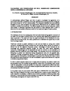
The following example is from
(Twomey and Smith 1993a, 1995). The pattern classification problem is a well known two class classification problem depicted in Figure 1. Two Gaussian distributions are classes A and B, where class A has a mean of 0 and a standard deviation of 1 and class B has a mean of 0 and a standard deviation of 2. There is considerable overlap between the classes, making this is a straightforward “hard” pattern classification task. Both training and testing sets contained equal numbers of observations from each class. Figure 1 here. Typically, networks are trained to decreasingly lower training tolerances in an attempt to achieve the “best” performing network. This assumes that lower training tolerances equate with improved performance, which is certainly not always the case.
To examine the relative
differences between RMSE and MAE, several networks were trained and tested in order to measure the effects of lowering the training tolerance for the two pattern classification problem where the correct output for class A is 0 and the correct output for class B is 1. A total of 13 different networks were trained, each to a different training tolerance. Training tolerances ranged from 0.08 to 0.6 for normalized input between 0 and 1. During training, a response was considered correct if the output was within a pre-specified absolute training tolerance of the target value (0 or 1). Training iterations continued for each network
5
until each of the training samples was deemed correct according to the specified training tolerance. Note that the tolerance that was used to train the network is an upper bound to the final training tolerance of the trained network, since the maximum acceptable error is applied to the worst training vector. Figure 2 is a plot of RMSE vs. training tolerance for the test set of 1000. This plot indicates that the RMSE resulting from networks trained at tolerances between 0.08 and 0.13 vary to some degree about a RMSE of 0.14. The RMSE for networks trained to tolerances from 0.14 to 0.40 steadily declines to a minimum of 0.11. At training tolerances of 0.5 and 0.6 there is a sharp increase to a RMSE of 0.24. The result of the mid-range training tolerances having the smallest RMSE is not expected. Minimum RMSE is often used as a criteria for determining the best trained network. Based on this criteria, the network trained to a tolerance of 0.4 would be chosen as the best performing among all those trained. This inconsistent phenomenon will be explained below. Figure 2 here. Figure 3 is a plot of the test set results for Mean Absolute Error (MAE) vs. training tolerance. These results, aside from some slight variations at the lower training tolerances, are closer to what is usually predicted: a steady decrease in MAE with a decrease in training tolerance. Criteria for selecting the best trained neural network is, again, to choose the network with the smallest MAE, in this case a training tolerance of 0.1. Figure 3 here. In order to explore these issues, the relative frequency histograms of test set residuals, or output errors, were constructed for each network. Six distributions that are representative of the 13 networks are presented in Figure 4. The network trained at a 0.1 training tolerance exhibits a trimodal distribution of errors. The large center peak indicates very small errors, or output that is very close to the targeted values. The smaller endpoint spikes denote clearly incorrect responses (i.e. a B signal for an A, or an A signal for a B); the right hand side shows a larger proportion of misclassifications for data sampled from class B, suggesting a harder classification task. There is a smaller proportion of errors in the region between the spikes, representing uncertain classifications (i.e. a 0.35 for A or a 0.65 for B). As the training tolerance increased, all three modes decrease until the error distribution takes on a Gaussian like distribution shape at tolerance of 0.4. At tolerances of 0.5 and 0.6, the distributions become bimodal with an increase
6
in distance between the modes at a tolerance of 0.6. At these large training tolerances, more vectors are classified in the less sure region because the networks have not been allowed to learn the classification model. Therefore, the RSME (and similarly, the MSE) penalizes distant errors, i.e. clear misses, more severely and therefore favors a network with few or no distant errors. This can cause networks with many uncertain predictions to have a lower RSME than a network with a few clear misses. MAE takes large errors into account, but does not weight them more heavily. Figure 4 here. 2.2 Specific Pattern Classification Error Metrics In pattern classification, interpretive schedules or rules are employed for classifying a correct response to a given input vector, i. This is because there is a discrete (generally binary or ternary) target but an analog output (generally between 0 and 1). For example, where the targets are either 0 or 1, it must be decided how to classify an output such as 0.65. There are two commonly used interpretive schedules for binary output, where subscript p is the number of patterns and there is a single output j per input vector i. For interpretive schedule I: if |op - tp| < 0.5 then Cp = 1, else Cp = 0
(4)
and for interpretive schedule II: if |op - tp| < 0.4 then Cp = 1, else Cp = 0
(5)
where Cp = 1 signals that pattern p belongs in class C and Cp = 0 signals that pattern p does not belong in class C. Percent good (PG) classification is a measure of the number of correct classifications summed over all n patterns using one of the interpretive schedules from above:
PG =
100 ∑ (1− C − C ) n n
tp
p =1
op
(6)
The effect of interpretative schedule on the reported performance was investigated by (Twomey and Smith 1993a, 1995) on the two class classification problem shown in Figure 1. Their results are summarized below. Figure 5 is a plot of the test set results measured in terms of percent good (using interpretative schedules) vs. training tolerance. This plot displays two curves representing interpretive schedule I and interpretive schedule II. Since the output for these networks are binary (0,1), interpretive schedule I classifies all output less than 0.5 as
7
coming from class A and all output greater than 0.5 as coming from class B. For interpretive schedule II, an output less than 0.4 is classified as coming from class A and output greater than 0.6 is classified as coming from class B. Note that for interpretive schedule II, an output that falls between 0.4 and 0.6 is always counted as incorrect. In both methods the network with the highest proportion of correct responses would be deemed as the “better” network.
As
anticipated, the curve for schedule I is consistently greater than curve for schedule II since schedule II is a subset of schedule I and the networks themselves are identical. The preferred networks according to interpretive schedule I were trained using tolerances between 0.08 and 0.5, while training tolerances between 0.08 and 0.2 yielded the preferred networks according to interpretive schedule II. The choice of interpretive schedule allows the user to decide how close an output should be to correctly signal a classification. The most generous rule possible, interpretive schedule I, allows for the possibility that many uncertain classifications (i.e. outputs between 0.4 and 0.6) will be considered correct, while the network may in fact have little or no knowledge of how to correctly classifying these input patterns. Figure 5 here. Martinez et al. (1994) derived an alternative pattern classification error metric, the absolute distance error (ADE) to quantify the normalized absolute distance from the highest activated class to the correct class using an ordered set of classes, e.g. a sequenced set of categories. This normalization is needed because in some cases the highest activated class is not equal to 1. ADE is defined as: m
ADE =
∑ ( c * oc )
c =1
m
∑ oc
− ca
(7)
c =1
where c is the class number using a scale of 1 to m, oc is the network output for a class c, and ca is the number of the actual (i.e. correct) class. This error captures how far away the predicted class is from the actual class, when the classes are ordered.
8
2.3 Classification Errors The relative importance of Type I and Type II errors are now considered for pattern classification networks. A two class problem defines the probabilities (p) of each type of error: p(Type I error) = α = p(Class B | Class A) and p(Type II error) = β = p(Class A | Class B). In many statistical models and neural network models the objective is to minimize the sum of these relative errors. However, some models will prefer to minimize Type I errors while others will prefer to minimize Type II errors, within some reasonable constraint on the other error type rate. In neural networks, the interpretive schedules discussed above may not meet the desired objective. In addition, networks are generally trained with the implicit, and perhaps the unrecognized, assumption that α = β. To enable the explicit consideration of the relative seriousness or cost of committing each type of error, an interpretive schedule strategy taken from statistical discriminant function analysis (Draper and Smith 1981) was proposed by (Twomey and Smith 1993a): locate the optimal boundary which discriminates between the two classes. The optimal boundary is the boundary point between classes used in the interpretive schedule which produces the desired levels of α and β errors. For the problem considered, it was assumed the desired outcome was to minimize the sum of α and β errors. A single network was trained on the pattern classification problem shown in Figure 1 to a tolerance of 0.1. Figure 6 is a plot of test set percent error vs. interpretive schedule. Total percent error is equal to the sum of Type I and Type II errors. The plot indicates that the minimal error occurs at a boundary point between classes equal to 0.3, that is output < 0.3 is considered class A while output > 0.3 is considered class B. This interpretive schedule produces minimal errors and is appropriate where the seriousness of committing a Type I error is equivalent to that of a Type II error. Note that this decision of interpretive schedule boundary point is made after the network is trained. Figure 6 here. To demonstrate the relationship of α to β, and to examine the effects of weighing the relative seriousness of one error type more heavily than the other, a plot of percent test set error vs. interpretive schedule is shown in Figure 7. The solid line represents percent incorrect classifications of Class A or Type I error (α). The dotted line represents percent incorrect
9
classifications of Class B or Type II error (β).
The plot indicates that as α decreases, β
increases. The lines intersect at decision boundary 0.2, where percent error is 0.17 for both error types. The ratio, or relative seriousness of Type II error to Type I error, is 1.0. Moving the decision boundary from 0.2 to 0.1 decreases the ratio of a Type II error to Type I error from 1.0 to 0.6. Moving the decision boundary in the opposite direction toward a value of 0.9 increases the ratio from 1.0 to 6.3, where the chances of committing a Type II error is more than 6 times as great as committing a Type I error; i.e. at 0.9, a Type I error is much less likely to occur than a Type II error. At 0.3, where the minimum sum of the two errors occurs, the ratio of Type II to Type I errors is 1.5. For interpretive schedule I, where the decision boundary occurs at 0.5, it is incorrectly assumed that both type of errors are given equal importance. In fact there are more than two times as many Type II errors as Type I errors at a value of 0.5. Figure 7 here. This plot illustrates how the decision boundary of the classification schedule can be adjusted a posteriori to reflect the relative seriousness of Type I vs. Type II errors for a given neural application. In fact it demonstrates that error type curves must be examined to ascertain the relative proportion of classification errors to be expected for the model under consideration. Reliance upon an implicit assumption of α = β will usually prove false when the actual trained network and its classification error characteristics are investigated.
3. Analysis of Residuals
Statistical model builders check residual plots, and neural network model builders should do likewise. The residual, or error, for pattern p is simply the target minus the network output:
r p = op − t p
(8)
There are three primary discoveries to be made from residual plots. These are discussed in turn. The first phenomenon to look for on a residual plot is bias.
Bias is a systematic
distribution of the residuals. In neural networks, bias often takes the form of undershoot or overshoot. Undershoot is where the network model does not reach the upper and lower extremes of the target data. Overshoot is the opposite phenomenon. Undershoot is a more frequently
10
found bias, especially for networks using the popular sigmoid transfer function, and can often be remedied by retraining the network on an expanded normalization range. Another form of bias is disproportionate errors on exemplar vectors or classes with under-representation, such as outliers or rare events. When the training data set includes classes or instances which happen relatively rarely in the training set, the neural network will often train to the dominant class(es), producing poor performance on the rarer class(es). This can be remedied by focused training on the rarer class(es), that is by artificially increasing their share of training vectors. An articulated architecture which is not globally connected, can also equalize performance among classes. In a globally connected architecture, such as the popular multilayered perceptron, all weights will be affected by all input patterns. This will cause dominant patterns or classes to dominate weight training.
An articulated architecture where certain
weighted connections are allocated to individual patterns or classes will alleviate this dominance problem. Such architectures which use supervised training include the probabilistic network and the cascade correlation network. The second phenomenon which can be easily recognized using residual plots is relative magnitude of individual errors. This was discussed in the earlier section where the squared error term (RMSE or MSE) was more favorable to many small errors than to a few large errors. The application will dictate which kinds of errors are permissible, but the modeler will want to check on distribution of the errors. Sometimes, a well performing network will produce a few large errors (clear misses) for outlying data points. These outliers can be further investigated for correctness and appropriateness to the model. The third aspect of residual analysis is related to the second. Residual plots of the testing and training sets must be compared. While it is expected that the overall magnitude of the error for the training set will be as low or somewhat lower than that of the testing set, both distributions should behave similarly. Significantly different residual distributions of training and testing errors can indicate bias in either or both of the data sets (i.e., the sets are inherently different from each other), or too small of a sample in one or both sets. Also, a large increase of magnitude of error from the training set to the testing set can be indicative of overtraining, i.e. memorization of the training set with poor generalization ability. Many remedies have been published addressing overtraining (also called overfitting). These include reducing the network
11
size, pruning trained connections with small weights, and ceasing training before the test set error significantly degrades.
4. Validation With Sparse Data
Neural network validation is especially problematic when dealing with sparse data where the decision on how to best use the limited data - for model construction or for model validation - is critical. Validation still needs improved methodologies for the neural network community, however there is a corresponding body of literature on validation of statistical models such as regression or discriminant function analysis (Mosier 1951, Stone 1974, Lachenbruch and Mickey 1968, Efron 1982, Efron 1983, Gong 1986). Several resampling methods have been developed which have two important aspects. First they use all data for both model construction and model validation. Second they are nonparametric techniques and do not depend on functional form or probabilistic assumptions. Below, after describing the two most common methods of neural network validation, these resampling methods are briefly described. 1. Resubstitution - resubstitutes the data used to construct the model for estimating model error, i.e. this is the training set error. Therefore the estimate of True Error equals the Apparent Error, and Bias is assumed to equal zero. Resubstitution is sometimes used in neural network validation, however it is usually noted to be biased downward (sometimes severely). It does use all of the data for both model construction and model validation, and requires only one model to be constructed. 2. Train-and-test - divide the data set into two sets. Use one set to construct the model (train the neural network) and use the other set to validate the model (test the neural network). This is the most common method of neural network validation. True Error is estimated directly as the testing set error, and Bias could be calculated by subtracting off the Apparent Error (training set error) from the testing set error. The proportion set aside for training of the available data has ranged, in practice, from 25% to 90%. The training set error (and therefore the estimate of True Error) is highly dependent on the exact sample chosen for training and the exact sample chosen for testing (which are completely dependent on each other since they are mutually exclusive). This creates a highly variable estimate of True Error, especially for small sample sizes. A
12
modification of this method is to divide the data into three sets - a training set, a first testing set used during training and a second testing set used for validating the trained network. The first testing set is used during training to decide when training should cease, that is, before overfitting takes place. The second testing set is used to estimate the True Error of the trained network. This method may result in a better generalizing final network, but the available data sample is divided three ways instead of two ways, decreasing the number of data points used for model construction. For both versions of train-and-test, only one model is constructed, but both training and testing are done on a subset of the available data. 3. Grouped cross validation - divides the available data into k groups. A total of k models are then constructed, each using k-1 data groups for model construction, and the hold out group for th k model validation. A final model which is used for application is built using all the data. True
Error is estimated using the mean of testing set errors of the k grouped cross validation models. This method uses all available data for both model construction and model validation, but requires the construction of k+1 models, i.e. training k+1 neural networks. Bias is estimated by subtracting the Apparent Error of the application network from the estimate of True Error. 4. Grouped jackknife - this is identical to the grouped cross validation except the Apparent Error is determined by averaging the Apparent Errors of each jackknifed model. (Where each jackknifed model is the same as each grouped cross validated model, described in the preceding paragraph.)
The Bias is then estimated by subtracting this new Apparent Error from the
estimated True Error. Therefore, the validation using grouped cross validation and grouped jackknife will be identical except for the calculation of Apparent Error. 5. Bootstrap - a data set of size n is drawn with replacement from the original data set of n observations. This sample constitutes the bootstrap training set. The bias of each bootstrapped network is estimated by subtracting the Apparent Error of that network (training set error) from the error of the network evaluated on the original total data set. This is repeated b times, each with a different randomly drawn data set. The overall estimate of Bias is obtained by averaging over the b estimates of bias. The final application model is constructed using all of the data, therefore b+1 models are constructed, i.e. b+1 neural networks are trained. True Error is estimated by adding the estimate of Bias to the Apparent Error of the application model. The
13
bootstrap is generally noted to be less variable than the grouped cross validation or grouped jackknife, but it can be downwardly biased. A simple example of the performance and variability of these methods on a one variable function approximation problem, previously used in both the statistical and the neural network literature for validation research, was presented by (Twomey and Smith 1993b). A total of N=1010 (x, y) observations were generated according to: y = 4. 26( e − x − 4 e −2 x + 3e −3 x ) ; x ranged from 0.0 to 3.10 (see Figure 8). Ten observations were randomly selected to make up the training and validation sample, n=10. The remaining 1000 observations were set aside as the true estimate of Bias. The prediction models, fully connected feedforward multi-layer networks, were all constructed of 1 input node (x variable), 1 hidden layer of 3 nodes and 1 output node (y). All networks were trained using the standard backpropagation algorithm. Training was terminated when either all training pairs were deemed correct within 10% of the targeted output, or after 10,000 presentations of the training sample. The error metric for testing was mean squared error (MSE). Figure 8 here. The standard method of train-and-test was considered first.
Twenty percent (2
observations) of the sample were removed for testing and the remaining 80% (8 observations) were used for training. To examine the variability of the Bias estimate, 45 networks, each with a different combination of train/test (8/2) samples, were trained and tested according to the method described above. True Bias was evaluated for each of the 45 networks over the 1000 observations. The results, shown in Table 1, indicate that model Bias estimated according to the train-and-test methodology, β$ T-T , on average over estimates the true model Bias and is highly variable. Considering the 10 observations chosen as the total sample for training/testing, this result is not surprising. It does illustrate the potential problems associated with the standard train-and-test methodology; that is - model performance can be highly dependent on which observations are chosen for training/testing. This can best be seen in Figure 9, where the True Error and Test Set Error (MSE) are plotted for each of the 45 networks. This plot illustrates that Test Set Error can under estimate the True Error approximately 50% of the time and over estimate the True Error approximately 50% of the time, sometimes drastically missing True Error.
14
Table 1 here. Figure 9 here. The resubstitution, cross validation, jackknife and bootstrap methods were also examined using the same sample of 10 observations.
In order to make the computational effort
comparable, 10 bootstrap samples (b=10) were constructed and the group size (k) of the cross validation and the jackknife was set to 1. Thirty additional bootstrap samples (b=40) were constructed to examine the effects of increased b. True Bias was again evaluated over the 1000 observations. The results are shown in Table 2. The Apparent Error estimate of Bias, obtained by the resubstitution method, under estimated True Bias, however it was the closest estimate and only required the construction of single network. The bootstrap method (b = 40) gave the next closest estimate of Bias, but with the highest computational effort of 41 total networks constructed. Table 2 here. The resampling methods have been shown to be superior to the train-and-test and resubstitution methods when used in statistical prediction models under conditions of sparse data (Mosier 1951, Stone 1974, Lachenbruch and Mickey 1968, Efron 1982, Efron 1983, Gong 1986).
Clearly, more research is needed to fully investigate the usefulness of resampling
methodologies for neural network validation when constrained by small samples. The main point is that if data is the primary constraint, then it may be prudent to expend more computational effort for construction and validation of multiple networks, and construct the final neural network model using all the data for training.
5. Conclusions
Because neural networks are purely empirical models, validation is critical to operational success. Most real world engineering applications require getting maximal use of a limited data set. Careful selection of an error metric(s) will ensure that the error being minimized is in fact the one most applicable to classification or approximation problem at hand. The trained network must be examined for signs of bias, even if error tolerances are met. Identification of bias will alert the user so that the network can be modified, or its outputs altered to reflect the known bias. Residuals of the training and testing sets can warn the user of the phenomena of overtraining and
15
overfitting. When using an interpretive schedule because of discrete target outputs, care must be taken to ensure the proper balance of Type I and Type II errors. In sparse data situations, a resampling methodology will allow all the data to be used to construct (train) the final operational neural network, while still providing for validation. The size of the groups in grouped cross validation or grouped jackknife, and the number of bootstrapped samples will depend on the computational resources available, the data set size and the precision needed in the validation step.
The resampling methodologies do expend
significantly greater resources in training and testing the neural networks, so in cases of ample data, the traditional train-and-test method may be the best choice.
16
REFERENCES Draper, N. R. and Smith, H. (1981). Applied Regression Analysis. New York: Wiley and Sons. Efron, B. (1982). The Jackknife, the Bootstrap, and Other Resampling Plans. SIAM NSFCBMS, Monograph 38. Efron, B. (1983). Estimating the error rate of a prediction rule: Improvement over crossvalidation. Journal of the American Statistical Association 78, 316-331. Gong, G. (1986). Cross-validation, the jackknife, and the bootstrap: Excess error estimation in forward logistic regression. Journal of the American Statistical Association 81, 108-113. Lachenbruch, P. and Mickey, M. (1968). Estimation of error rates in discriminant analysis. Technometrics 10, 1-11. Martinez, S., Smith, A. E. and Bidanda, B. (1994). Reducing waste in casting with a predictive neural model. Journal of Intelligent Manufacturing 5, 277-286. Mosier, C. I. (1951). Symposium: The need and the means of cross-validation. I. Problem and designs of cross-validation. Education and Psychological Measurement 11, 5-11. Stone, M. (1974). Cross-validory choice and assessment of statistical predictions. Journal of the Royal Statistical Society Series B 36, 111- 147. Twomey, J. M. and Smith, A. E. (1993a). Power curves for pattern classification networks. Proceedings of the 1993 IEEE International Conference on Neural Networks, 950-955. Twomey, J. M. and Smith, A. E. (1993b). Nonparametric error estimation methods for the evaluation and validation artificial neural networks. Intelligent Engineering Systems Through Artificial Neural Networks: Volume 3 ASME Press, 233-238. Twomey, J. M. and Smith, A. E. (1995). Performance measures, consistency, and power for artificial neural network models. Journal of Mathematical and Computer Modelling 21, 243258.
17
Weiss, S. M., and Kulikowski, C. A. (1991). Computer Systems that Learn. San Mateo, CA: Morgan Kaufmann Publishers, Inc.
18
0.4
CLASS A
CLASS B
0.3
0.2
Y
0.1
0 -8
-4
0
X
4
Figure 1. Two Class Classification Problem.
19
8
RMSE OF TEST SET
0.5
0.4
0.3 0
0.1
0.2
0.3
0.4
0.5
TRAINING TOLERANCE
Figure 2. RMSE as a Metric for Selecting the Best Trained Network.
20
0.6
0.6
MAE OF TEST SET
0.5 0.4 0.3 0.2 0.1 0
0.1
0.2
0.3
0.4
0.5
0.6
TRAINING TOLERANCE
Figure 3. MAE as a Metric for Selecting the Best Trained Network.
21
TRAINING TOLERANCE .1 0.4
0.3
RELATIVE FREQUENCY 0.2
0.1
0 -1
-0.6
-0.2
0.2
0.6
1
ERROR
TRAINING TOLERANCE .4 0.4
0.32
RELATIVE FREQUENCY 0.24
0.16
0.08
0 -1
-0.6
-0.2
0.2
0.6
1
ERROR
TRAINING TOLERANCE .5 0.4
0.3
RELATIVE FREQUENCY 0.2
0.1
0 -1
-0.6
-0.2
0.2
0.6
ERROR
Figure 4. Relative Frequency Histograms of Residuals.
22
1
1 Schedule I PG OF TEST SET
0.8 0.6 Schedule II 0.4 0.2 0 0
0.1
0.2
0.3
0.4
0.5
0.6
TRAINING TOLERANCE
Figure 5. Performance According to Percent Good Interpretive Schedules.
23
TOTAL TEST SET PERCENT ERROR
25 23 21 19 17 15 0
0.2
0.4
0.6
0.8
BOUNDARY POINT
Figure 6. Minimization of the Sum of α and β.
24
1
PERCENT TEST SET ERROR
40 35 30
Type II Error
25 20 15 Type I Error
10 5 0 0
0.2
0.4
0.6
0.8
1
BOUNDARY POINT
Figure 7. The Effects of Changing the Decision Boundary on Relative Errors.
25
0.4 0.2 0
Y
-0.2 -0.4 -0.6 -0.8 -1 X
Figure 8. Function Approximation Problem: y = 4. 26( e − x − 4 e −2 x + 3e −3 x ) .
26
TEST
TRUE
0.5
0.4
MSE
0.3
0.2
0.1
0 1
6
11
16
21
26
31
36
41
NETWORK NUMBER
Figure 9. True and Test Set Error According to Train-and-Test Method. (Data Sorted by True MSE.)
27
45
Table 1. Results of Train-and-Test Methodology.
Mean Variance
Apparent Error Estimated Bias 0.016 0.075 4.3E-05 0.016
28
True Bias 0.028 0.001
Table 2. Estimates of Bias from Resampling Methodologies Compared to Resubstitution and Train-and Test.
Bias # Networks
True 0.013 -
Apparent 0.00 1
CV (k=1) 0.065 11
Jack (k=1) 0.058 11
29
Boot (b=10) 0.037 11
Boot (b=40) 0.034 41