natural resource management - the GeoWEPP example ... models originally developed for small-scale, site ..... The mapping based on a relative value allows.
Implementing a process-based decision support tool for natural resource management - the GeoWEPP example Chris S. Renschler a and Dennis C. Flanagan b a
Dept. of Geography, University at Buffalo - The State University of New York, Buffalo, NY 14261, USA b
U.S. Dept. of Agriculture National Soil Erosion Research Laboratory, West Lafayette, IN 47907, USA
Abstract: Practical decision-making in spatially distributed natural resource management is increasingly based on process models linked to Geographical Information Systems (GIS). Geo-spatial environmental data and decision support tools can now be made available to a much larger audience by using powerful personal computers and internet-accessible mapping tools. Traditionally decision support tools based on process models were not typically developed for applications across a wide range of spatial and temporal scales of interest, utilizing commonly available data of variable precision and accuracy, and Graphical User Interfaces (GUIs) to communicate with a diverse spectrum of users with different levels of expertise. To implement such scientifically accepted and highly sophisticated models and avoid poor decision making by a diverse group of users based on inaccurate results derived by applying the model at an inappropriate scale, or by using data of insufficient precision or accuracy, it is critical to develop a scientific and functional strategy to successfully design, implement and apply such geo-spatial decision support tools. GUIs play a key role in communicating effectively between the model developer and user in describing data and model scales, as well as GIS methods for transformation of information between scales, that produce useful assessment results at the user’s scale of interest. This paper presents a strategy and a scaling theory that are implemented in developing a geo-spatial natural resource management tools for the Water Erosion Prediction Project (WEPP). The Geo-spatial interface for WEPP (GeoWEPP) accounts for fundamental processes, model and users needs, but also matches realistic data availability and environmental settings. Presently the GeoWEPP approach enables even the non-GIS-and-modeling-literate user to quickly assemble the model input data from a local or the WEPP database and geo-spatial data that is readily available through the Internet for any location in the contiguous US to start soil and water conservation planning. Keywords: Natural resource management; Geographic Information Systems; Decision support tools; Water erosion modeling 1.
INTRODUCTION
assumptions in model design, calibration and validation.
Environmental modeling and assessment are built in large part on an understanding of environmental properties and processes. Scientists and engineers traditionally approach this paradigm by constructing process models to understand and predict the inherent behavior of an environmental system and its behavior after a natural and/or anthropogenic impact. Depending on the scale of interest, this results in determining the most relevant physical parameters, equations, and model approaches that can be used as a basis for decisionmaking and the design of responses to specific environmental management challenges (Law and Kelton, 1991). Since such parameters, equations, and model approaches were developed for a particular problem, specific temporal and spatial scales, and input data of known quality, this context is used to justify explicit or implicit
2.
IMPLEMENTING PROCESS MODELS AND GIS FOR DECISION MAKING
Process-based models represent our most detailed scientific knowledge, usually considering properties and processes at small spatial and temporal scales, but have extensive data requirements, e.g. the Stanford Watershed Model (Crawford and Linsey 1966). In contrast to process models, which require a minimum of calibration but a large number of input parameters, empirical models require far less data, and are therefore easier to apply, but do not take full advantage of our understanding of process mechanics and have limited applicability outside conditions used in their development. Once released and publicized,
187
both types of models may end up being used (and misused) in a range of situations, across many spatial and temporal scales, and with data of varying quality (e.g. Wischmeier, 1976). A more rational approach is to design and evaluate models in anticipation so that these are tested for utilizing realistic data settings and application situations in mind. With increasing availability and use of geospatial data management tools, such as GIS, new issues have arisen with respect to spatial data, application of models to a range of spatial scales, and the role of spatial data handling tools and analytical techniques in decision making (Goodchild et al., 1993; Clarke et al., 2001). GIS software packages are designed for geo-spatial data assembling, processing, storage and visualization of input data and model output, and are used widely as analytical tools in environmental management (Burrough, 1986).
direction of scale change and requires methods such as interpolation and extrapolation or aggregation and disaggregation. The observed data that represent a true pattern of a natural property or process is being transformed through a sequence of necessary changes in scales inherent in the data preand post-processing in order to apply a spatial model assessment (Figure 1).
With increasing availability of powerful personal computers and public access to geo-spatial data sets through the Internet, it is common to see models originally developed for small-scale, site specific analyses now applied to new contexts, new problems, and, through GIS, to large areas to examine spatial variations in environmental impact (Pandey et al., 2000). Increasing ease of use and availability of environmental models, GISinterfaces and decision support tools has expanded the user base to include planners, farmers, politicians and environmental groups.
Figure 1. Scaling theory for implementing environmental assessment tools. Note that scaling and evaluation through scaling requires a transformation of information (=>) and within the domain of digital geo-spatial data handling (^^^).
While this represents an exciting opportunity to increase the scientific basis for decision-making, it raises important issues with respect to the manner in which models are developed, linked with geospatial tools such as GIS, and used at different scales (Nyerges 1993). 3.
The initial first ‘scaling’ of information about natural phenomena occurs as a function of the accuracy, precision and sampling strategies used in measuring processes and phenomena. Further scaling steps occur in data processing and modeling. Consequently, although the true pattern of a natural process at the true process scale has a true variance, both measured data and predictions have different process scales and variances. The ratios of measurement-to-process scales and modelto-process scales provide an indication of the degree of impact of the scale effect (Blöschl, 1999). Based on this theory, the presented extended scaling framework for decision-making (Figure 1) provides a foundation for addressing scaling issues in the design and use of models for practical decision-making.
SCALING THEORY
Therefore a scaling theory is critically important in an interdisciplinary approach to implement environmental process models that are developed at a particular scale. A new conceptual scaling theory is needed that defines scales of information for real patterns. The methods used to measure spatially and temporally variable environmental properties, to derive model input parameters, and to predict the processes represented by models may not necessarily be at the same scale as the environmental process assessment of interest. Even the scale transformations in modeling and model results itself may not be at the same scale as the final assessment. The term scale refers to a characteristic length or time and can be used either as a qualitative term (e.g. a small-scale process) or as quantitative measure in space dimensions (Blöschl, 1999). Scaling is thus a change in either spatial or temporal scale and has a certain direction and magnitude. Up and down scaling describes the
4. IMPLEMENTING A SCALING METHOD IN MODEL DESIGN 4.1 Model Design In using process models in decision-making the focus is basically on (i) the decision-maker's scales of interest (assessment results), (ii) availability of data sets that might support appropriate model applications (assessment base), and (iii) the choice of an model that is adequate for the decision-
188
making goals (see also Hoosbeek and Bryant, 1992) (assessment core). These three concurrent initial steps define the questions to be answered as well as the models and data sources to be used. In general, however, it is potential users’ scales of interest, and scales of readily available data that should drive model design or selection, as opposed to using or designing the most sophisticated process model as the starting point and then determining data needs and result scales.
transformation creates awareness and a level of user confidence that the interface handles data and model in an appropriate way. 4.2
Modern data handling in environmental assessment increasingly relies on vector-based (point and line features), raster-based or hybrid GIS (Figure 2) as the core of a data processing, analysis and display package that covers all of the scaling steps prior to final decision-making. The integrating role of GIS in environmental analysis system, and the tradition of using meta data and geospatial data standards in GIS makes tracking scaling steps much easier. The six data models used in GIS, based on point, line or raster features in space dimensions, each have advantages and disadvantages in representing a specific set of data in space (Meijerink et al., 1994), and again introduce scaling transformations in the assessment process. Appropriate data models for a particular application conserve the relevant information used to representing a certain environmental process or property with a minimum error. This can be achieved through careful consideration of the original data source and its uncertainty related measurement technique. This additional information helps in design scaling methods at the particular data scale and in analyzing the effects of scaling on model output and decisions The following example illustrates the implementation of the described scaling method into the Graphical User Interface (GUI) for a practical decision support tool in soil and water conservation.
Because appropriate geo-spatial assessment requires careful consideration of all the steps in integrating data, modeling and decision-making, each step in the scaling sequence (Figure 1) must be assessed in terms of how data are being transformed (scaled). If the management decision is not sensitive to the use of readily available aggregated data, there is no need to spend time and resources on collecting more detailed data. Thus, an additional benefit is that this assessment allows identification of areas where less sophisticated approaches or less restrictive data requirements might be used without compromising the final outcome of the decisionRegion
5.Scaling: Quality assessment
Watershed Farm Field
uncertainty assessment
Hillslope
post- 4.Scaling: Mapping processing of results
assessment answer
Plot scale
User’s scales of interest
Graphical User Interface
location visual ization
GIS
Single event additional data entry
Short-term Multiple events Long-term Historic data Scenario
1.Scaling: Commonly availability Common available pre-processing Database data
require ments
The Role of Geographical Information Systems
3.Scaling Modelapplication
assessment question 2.Scaling: Discretization
making process. 4.4
Figure 2. Structure of a proposed spatially distributed environmental assessment tool.
Process Modeling in soil and water conservation
One of the most known, applied and implemented approaches for estimating long-term average annual soil loss are the Universal Soil Loss Equation (USLE) (Wischmeier and Smith 1978) and the Revised Universal Soil Loss Equation (RUSLE) (Renard et al., 1997). Both are simple empirical equations based on factors representing the main processes causing soil erosion. USLE and RUSLE have proven to be practical, accessible prediction tools and were therefore implemented in the U.S. soil and water conservation legislation. However, these model approaches have been used and misused widely at various scales worldwide (Wischmeier 1976) and the implementation of a process-based erosion model is desirable.
Note that a Geographical Information System (GIS) stands for a geo-spatial tool to assemble, process, analyze and visualize environmental data. The GIS is the glue between the user’s scale of interest and the scales related to available process data and models. An integrated development of available data and tools (black compartments) and geo-spatial data handling procedures (white compartments) leads to a successful model application for decision-support.
However, such an assessment might also identify steps where data inaccuracy or transformations introduce error or uncertainty that are beyond tolerable levels in terms of the impact on final decision making. Explicit recognition of this helps reduce the risk of poor decision-making. It is important to recognize that the scaling steps can also be used as a framework for building a sequence of data transformations focused on providing results that are both adequate and accurate enough for the decision-maker’s scales of interest. Enabling the user to set certain thresholds for acceptance along this sequence of data
In contrast to these empirical model approaches, efforts in erosion process research in the U.S. led to the development of the process-based hillslope soil erosion model WEPP (Flanagan and Nearing, 1995). WEPP simulates climate, infiltration, water
189
balance, plant growth and residue decomposition, tillage and consolidation to predict surface runoff, soil loss, deposition and sediment delivery over a range of time scales, including individual storm events, monthly totals, yearly totals or an average annual value based on data for several decades. The publicly available WEPP model is a continuous distributed-parameter soil erosion assessment tool that can be applied to representative hillslopes and a channel network at small watershed scales (Ascough II et al., 1997). A comparison of the performance of WEPP with other state-of-the-art erosion models using common data sets showed that data quality is an important consideration and primarily process-based models not requiring calibration have a competitive edge to those in need of calibration (Favis-Mortlock, 1998).
The U.S. Geological Survey (USGS) Digital Elevation Models (DEM) and Digital Raster Graphs (DRG) at the 1:24,000 scale are then automatically imported and preprocessed. Based on the imported DRG and DEM scene, a channel delineation takes place based on the DEM in the next wizard step. Channel parameters and a watershed outlet cell have to be set in the wizard to delineate drainage pattern and a watershed with sub-catchments. The Topographical Analysis Software TOPAZ (Garbrecht and Martz, 2000) is integrated in the wizard. TOPAZ requires a Critical Source Area (CSA) and a Minimum Source Channel Length (MSCL) to derive a channel network. Before the model run, the wizard guides the user through various steps to set the required minimum model input parameters for WEPP provided by pick lists of the latest WEPP model (see also Flanagan and Nearing, 1995). The WEPP watershed simulation can be performed with two simulation methods (or both): (1) a relatively faster Watershed Method that allows one to simulate sediment yields from single representative hillslopes for each subcatchment with a channel routing for the watershed outlet (Figure 3) and (2) a longer Flowpath Method that allows one to simulate and merge soil loss along all possible flowpaths within the watershed, but without channel routing (Figure 4). [For more information about how to derive representative hillslopes as well as how to merge multiple flowpath simulations, refer to Cochrane and Flanagan (1999) or Flanagan et al. (2000).
4.5 The Geospatial Interface to the Water Erosion Prediction Project (GeoWEPP) A GIS-driven GUI is a user-friendly approach to combine a process model and the spatial capabilities of a GIS for practical assessment purposes and decision-support at a particular location (Renschler et al., 2000). To be useful and successful in its implementation and acceptance requires the use of widely available data sets and the automatic preparation of model default input parameters to begin controlled and reliable model predictions. The prototype of this GIS-based GUI the Geo-spatial Interface for WEPP (GeoWEPP) (Renschler, 2001) - is an interface for using WEPP through a wizard in the commercial GIS ArcView 3.2 for Windows 98, 2000 and NT. The currently released test version of GeoWEPP ArcX 1.0 beta is an ArcView project/extension that includes the scaling theory described in this paper. GeoWEPP starts as a user-friendly wizard that allows the user to go through four essential steps of the described scaling theory to derive topographical input parameters for a WEPP watershed simulation based on a DEM of one's own or alternatively from a publicly available data source: •
Import of Digital Elevation Models (Preprocessing for Database Scale)
•
Channel and Watershed Delineation (Discretization for Modeling Scale)
•
Model Input Parameters and Model Run (Modeling for Prediction Scale)
•
Mapping Model Results (Post-processing for Assessment Scale)
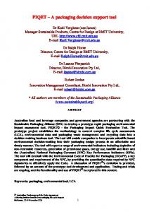
Figure 3. Model result post-processing: Watershed method: Off-site assessment (Sediment yields).
The GeoWEPP wizard itself is especially designed that even GIS beginners can handle the software. All the procedures and tools required to prepare all input data, run the model and visualize the results are included in the wizard.
Figure 4. Model result post-processing: Flowpath method: On-site assessment (Soil losses).
190
The WEPP model creates numerous outputs to its model components, including Climate Simulation, Subsurface Hydrology, Water Balance, Plant Growth, Residue Decomposition and Management, Overland Flow Hydraulics, Hillslope Erosion Component, Channel Flow Hydraulics, and Channel Erosion Surface. The current wizard allows you to visualize only a small portion of the WEPP model output such as runoff, soil loss, sediment deposition and sediment yield from hillslopes and channel segments. The average annual simulation results for the WEPP Watershed Method are displayed as text files and visualized as a map.
about data quality and uncertainties to users is an important first step, but insufficient. Given the known expertise level of most decision-makers, scaling theory encourages model developers to assess the impact of data quality and model assumptions on decision-making as an integral and basic part of model development. From the decision maker’s perspective, this approach will lead to efficient decision making based on data, models and processing steps that represent the least complex approach using the most easily obtained data to achieve results that are adequate for decision making.
The mapping based on a relative value allows flexible in setting a threshold for the assessment. Therefore the results are mapped as a relative measure to a tolerable soil loss or target value (T). The concept of a T value (Schertz, 1983) describes in theory the annual replacement rate for a soil type to maintain a sustainable land use. The Natural Resources Conservation Service (NRCS) implemented T that is determined for each location based on properties of root limiting subsurface soil layers, current climate regions and an economic feasibility summarized for soils in land resource regions. Relative to this T value, the results of soil loss and sediment yield are classified and displayed in green colors, intolerable results are shown in red, and deposition areas are in yellow (Figure 3 and 4).
6.
The U.S. Department of Agriculture National Soil Erosion Laboratory (USDA-ARS- NSERL) provided financial assistance for this work. The authors gratefully acknowledge the support of Dr. Bernard Engel, Purdue University. The authors thank Jim R Frankenberger, Thomas A Cochrane, and Roel C Vining for their contribution to the GeoWEPP project. 7.
REFERENCES
Ascough II JC, Baffaut C, Nearing MA, and Liu BY. The WEPP Watershed Model: I. Hydrology and erosion. Transactions of the American Society of Agricultural Engineers 40(4): 921-933. 1997. Blöschl G. Scaling issues in snow hydrology. Hydrological Processes 13: 2149-2175. 1999. Burrough PA. Principles of Geographical Information Systems for Land Resources Assessment. Oxford: Oxford University Press. 1986. Clarke KE, Bradley OP, and Crane M.P. Geographic Information Systems and Environmental Modeling. Upper Saddle River: Prentice Hall. 2001. Cochrane T, and Flanagan DC. Assessing water erosion in small watersheds using WEPP with GIS and digital elevation models. Journal of Soil and Water Conservation 54(4): 678-685. 1999. Crawford NH, and Linsley RK. Digital Simulation in Hydrology: Stanford Watershed Model IV (Dept. of Civil Engineering Tech Report). Stanford: Stanford University. 1966. Favis-Mortlock D. Validation of field scale soil erosion models using common datasets. In: Boardman, J., Favis-Mortlock, D., Modelling Soil Erosion by Water. NATO ASI Series I., Vol. 55, 89-127. 1998. Flanagan DC, and Nearing MA, editors. USDAWater Erosion Prediction Project Hillslope Profile and Watershed Model Documentation. NSERL Report No. 10, USDA-ARS
After assessing the effect of an initial land use scenario, the user may interactively change the land use to get acceptable T values for all watershed areas (Note that the GeoWEPP version presented here is for a single soil and land use in each subcatchment. Future versions are currently under development to include spatially distributed soil and land use along hillslopes). 5.
ACKNOWLEDGEMENTS
CONCLUSIONS
Any spatially distributed environmental modeling assessment approach in a geo-spatial domain requires five essential scaling steps to transform environmental realities in to decisions. Understanding and following this structure allows the efficient design and evaluation of spatially distributed model applications with a GIS, considering different scales of interest and related uncertainties in data collection and processing, modeling, and processing and representation of results. Scaling theory highlights weaknesses and strengths in geo-spatial environmental assessment approaches, and provides a framework for understanding scaling and uncertainty issues that are critical in supporting useful and accurate decision-making. The results presented in this paper provide strategies to optimize spatially distributed process models. Providing information
191
National Soil Erosion Research Laboratory, West Lafayette, Indiana. 1995. Flanagan DC, Renschler CS, and Cochrane TA. Application of the WEPP model with digital geographic information. In: Problems, Prospects and Research Needs. Proceedings of the 4th International Conference on Integrating GIS and Environmental Modeling (GIS/EM4); 2000 Sep 2-8; Banff, Alberta, Canada. 2000. Garbrecht J, and Martz LW. TOPAZ: An automated digital landscape analysis tool for topographic evaluation, drainage identification, watershed segmentation and subcatchment parameterization: Overview. ARS-NAWQL 95-1, USDA-ARS, Durant, Oklahoma. ; Accessed 2000 June 289. 2000. Goodchild MF, Parks BO, and Steyaert LT. Environmental modeling with GIS (Oxford University Press, Oxford. 1993. Hoosbeek MR, and Bryant J. Towards the quantitative modeling of pedogenesis: a review. Geoderma 55: 183-210. 1992. Law AM, and Kelton WD. Simulation modeling and analysis (McGraw-Hill, New York, ed. 2). 1991. Meijerink AMJ, de Brouwer HAM, Mannaerts CM, and Valenzuela CR. Introduction to the use of Georgaphical Information Systems for practical Hydrology (ITC Publication 23, Enschede), p. 34. 1994. Nyerges TL. Understanding the scope of GIS: Its relationship to environmental modeling. In Environmental modeling with GIS, M.F. Goodchild, B.O. Parks, L.T. Steyaert, Eds. (Oxford University Press, Oxford, 1993), pp. 75-93. 1993. Pandey S, Harbor J, and Engel B. Internet Based Geographic Information Systems and Decision Support Tools (Quick Study Series, URISA Publications, Chicago). 2000. Renard KG, Foster GR, Weesies GA, McCool DK, and Yoder DC. Predicting Rainfall Erosion Losses - A Guide to Conservation Planning with the Revised Universal Soil Loss Equation (RUSLE). U.S. Dept. of Agriculture, Agricultural Handbook 703. 404 p. 1997. Renschler CS. GeoWEPP - The Geo-spatial interface for the Water Erosion Prediction Project WEPP). 2001. ;. Accessed 2001 November 1. Renschler CS, Engel BA, and Flanagan DC. Strategies for implementing a multi-scale assessment tool for natural resource management: a geographical information science perspective. In: Problems, Prospects and Research Needs. Proceedings of the 4th International Conference on Integrating GIS
and Environmental Modeling (GIS/EM4); 2000 Sep 2-8; Banff, Alberta, Canada. 2000. Schertz DL. The basis for soil loss tolerance. Journal of Soil and Water Conservation 38 (1), 10-14. 1983. Wischmeier WH. Use and misuse of the universal soil loss equation. Journal of Soil and Water Conservation 31 (1): 5-9. 1976. Wischmeier WH, and Smith DD. Predicting Rainfall Erosion Losses - A Guide to Conservation Planning. U.S. Dept. of Agriculture, Agricultural Handbook 537. 85 p. 1978.
192