KeywordsâSensor Fusion, Kalman Filter, Gyroscope,. Accelerometer, Magnetometer, Tilt Compensation. I. INTRODUCTION. Or
Implementing a Sensor Fusion Algorithm for 3D Orientation Detection with Inertial/Magnetic Sensors Fatemeh Abyarjoo1, Armando Barreto1, Jonathan Cofino1, Francisco R. Ortega2 1
Electrical and Computer Engineering Department. Florida International University. Miami, FL. USA 2 School of Computing and Information Science. Florida International University. Miami, FL. USA. {fabya001, barretoa, jcofi001, forte007}@fiu.edu
Abstract— In this paper a sensor fusion algorithm is developed and implemented for detecting orientation in three dimensions. Tri-axis MEMS inertial sensors and tri-axis magnetometer outputs are used as input of fusion system. A Kalman filter is designed to compensate the inertial sensors errors by combining accelerometer and gyroscope data. A tilt compensation unit is designed to calculate the heading of the system.
II. DATA ACQUISITION Our system is composed of a tri-axis gyroscope, a tri-axis accelerometer and a tri-axis magnetometer. Our sampling rate is 8.96 samples per second. The gyroscope resolution is 16 bits and the sensitivity is 0.007˚/sec/digit. The accelerometer sensitivity is 0.00024g/digit. Raw data were acquired while the sensors were stationary on the desk. In Figure 1, the raw data extracted from sensors are shown.
Keywords—Sensor Fusion, Kalman Filter, Gyroscope, Accelerometer, Magnetometer, Tilt Compensation
I. INTRODUCTION Orientation tracking has a wide range of applications including military, surgical aid, navigation systems, mobile robots, gaming, virtual reality and gesture recognition [1], [2]. So far, orientation detections are mostly done by using an “externally referenced” [3] motion sensing technologies, for example video, radar, infrared and acoustic. Although these methods achieved good results in an indoor environment, they suffer from some limitations, like shadows, light interruptions, distance limitations and interference [4], [5]. An alternative approach is to use inertial sensors. Inertial sensors detect physical quantities of the moving object regardless of external references, environment lighting or friction. This detected movement is directly related to object, which sensors are attached on. Furthermore, inertial sensors are the self-contained technology which do not need external devices, like cameras or emitters. These sensors have been used in submarines, spacecraft and aircrafts for many years [6]. Micro-Electro-Mechanical-System (MEMS) based inertial sensors have emerged during last decade. Due to their miniature size, low power consumption, and light weight [7], the use of inertial MEMS sensors has developed rapidly in recent years. In this paper, an algorithm is proposed to detect orientation in three dimensions. The inertial measurement unit (IMU) is composed of a tri-axis gyroscope, a tri-axis accelerometer, and a tri-axis magnetometer. A Kalman filter is implemented to yield the reliable orientation. Tilt compensation is applied to compensate the tilt error.
Figure 1: Raw data The raw data are not ready to use and they need to be calibrated. To calibrate these data, scale and bias must be taken into account. The bias represents how far the center of data is from the zero. The scale means how much larger the range of data from the sensor is than the real meaningful data. Figure 2 presents the calibrated data from the gyroscope, the accelerometer and the magnetometer respectively. It can be observed that in the accelerometer calibrated data, X and Y axes are approximately zero and the Z-axis is -1. The axes X and Y are zero because there is no acceleration in these axes. In fact, the only acceleration present is the earth’s gravity, which is along the Z-axis pointed downward. This is the reason for measuring a negative number in the Z-axis. The hardware was stationary when the data were recorded and no rotational movement was applied to the
system. Therefore, the gyroscope did not record rate of rotation. The fluctuations which are seen are white noise. This noise is inseparable from the gyroscope data; it will cause the drift in the rotational angle, which is obtained based on the gyroscope’s data.
Trapezoidal integration method equation [8] is shown in equation 1. � 1 � f�x�dx = �b − a�f�a� + �b − a�[f�b� − f�a�] 2 �
(1)
The computed result drifts over time and after approximately 30 seconds it drifts down about 50 degrees. The explanation for this phenomenon is that the integration accumulates the noise over time and turns noise into the drift, which yields unacceptable results. In fact, the integration result is less noisy than the gyroscope signal but there is more drift present. One good aspect of the gyroscope is that it is not affected by earth’s gravity.
Figure 2: Calibrated data III. METHOD MEMS gyroscopes use the Coriolis acceleration effect on a vibrating mass to detect angular rotation. The gyroscope measures the angular velocity, which is linear to rate of rotation. It responds quickly and accurately and the rotation can be computed by time-integrating the gyroscope output. Figure 3 depicts the rotational angle, which is obtained by the trapezoidal integration from the gyroscope signal.
Accelerometers measure linear acceleration based on the acceleration of gravity [9]. The problem with accelerometers is that they measure both acceleration due to the device’s linear movement and acceleration due to earth’s gravity, which is pointing toward the earth. Since it cannot distinguish between these two accelerations, there is a need to separate gravity and motion acceleration by filtering. Filtering makes the response sluggish and it is the reason why the accelerometer is mostly used by the gyroscope. By utilizing the accelerometer output, rotation around the X- axis (roll) and around the Y-axis (pitch) can be calculated. If Accel_X, Accel_Y, and Accel_Z are accelerometer measurements in the X-, Y- and Z-axes respectively, equations 2 and 3 show how to calculate the pitch and roll angles: Accel_X Pitch = arctan � � �Accel_X�� + �Accel_Z�� Accel_Y Roll = arctan � � �Accel_Y�� + �Accel_Z��
�2� �3�
These equations provide angles in radians and they can be converted to degrees later. Figure 4 presents the rotation angle, which is computed by using the accelerometer signal. Despite recording this signal in a much longer interval, contrary to Figure 3, no drift is observed in Figure 4, but it is noisier.
Figure 3: Drifting Rotation angle calculated by the Gyroscope integration
A. Kalman Filter Kalman filtering is a recursive algorithm which is theoretically ideal for fusion the noisy data. Implementation of the Kalman filter calls for physical properties of the system. Kalman filter estimates the state of system at a time (t) by using the state of system at time (t-1). The system should be described in a state space form, like the following: %&'( = )%& + *& ,& = -%& + .&
Figure 4: Noisy Rotation angle calculated by the Accelerometer In order to measure rotation around the Z-axis (yaw), the other sensors need to be incorporated with the accelerometer. It has now been observed that neither the accelerometer nor the gyroscope provides accurate rotation measurements alone. This is the reason to implement a sensor fusion algorithm to compensate for the weakness of each sensor by utilizing other sensors. IV. SYSTEM CONFIGURATION The applied sensor fusion system is depicted in Figure 5. The calibrated accelerometer signal is used to obtain roll* and pitch* by equations 2 and 3. Roll* and pitch* are noisy calculations and the algorithm combines them with the gyroscope signal through a Kalman filter to acquire clean and not-drifting roll and pitch angles. On other hand, a tilt compensation unit is implemented, which uses a magnetometer signal in combination with roll and pitch to calculate the challenging yaw rotation.
�5�
Where; %& is the state vector at time k, A is the state transition matrix, *& is the state transition noise, ,& is measurement of x at time k, H is the observation matrix and .& is the measurement noise. State variables are the physical quantity of the system like velocity, position, etc. Matrix A describes how the system changes with time and matrix H represents the relationship between the state variable and the measurement. In our Kalman filter input vector is defined as follows: ω (6) x = 0 φ3 1 −∆t (7) 3 A=0 0 1 (8) H=[1 0] Where 7 is the angular velocity from the gyroscope, and ϕ is the rotation angle, which is calculated by the accelerometer signal. To implement the Kalman filter, the steps in algorithm 1 should be executed [10]. The A, H, Q and R should be calculated before implementing the filter. Q and R are covariance matrices of *& and *& respectively, which are diagonal matrices. 8& is the system measurement and %9& is the filter output. Algorithm 1 1.
Figure 5:System Structure
�4�
Set initial values, :; = 0, %9; = 0 2. State prediction; the superscript ‘-‘means predicted value. This step uses the state from the previous time point to estimate the state at the current time point. %9&< = )%9&