Tutorials in Quantitative Methods for Psychology 2007, Vol. 3(1), p. 8-13.
Implementing and evaluating the nested maximum likelihood estimation technique
Denis Cousineau Université de Montréal Estimating parameters describing response time distributions is difficult. The most commonly used method for parameter estimation is the maximum likelihood method (ML). However, this method applied on the three-parameter Weibull distribution returns biased estimates and the amount of bias is unknown. A recent method, that we call nested maximum likelihood, was proposed by Gourdin, Hansen and Jaumard (1994). Due to its complexity, it has never been used and tested systematically. Here I compare it to the maximum likelihood method. The results shows that nested maximum likelihood is slightly better than ML. Although the gains are marginal, the method has important implications for future research in parameter estimation.
Statistical methods in psychology are dominated by the normal distribution. However, very few measures in experimental psychology follow this distribution. For example, the time to complete a task (maybe the most direct access to cognitive processes) is always asymmetrical with a long tail to the right (e. g. Cousineau and Shiffrin, 2004, Hockley, 1984, with an exception, Hopkins and Kristofferson, 1980). Hence, it is of prime importance that we move towards a description of the response times (RTs) that acknowledge this asymmetry. The most natural such description assumes that there is a true minimum RT below which it is not possible to respond (fast-guessing notwithstanding). Then, three convenient descriptors could be: the lowest possible RT, the width of the distribution and the degree of asymmetry. See Rouder, Lu, Speckman, Sun and Jiang (2005) for reasons supporting this choice. Whereas the width is akin to standard deviation,
We would like to thank Sébastien Hélie for his comments on an earlier version of this text. Request for reprint should be addressed to Denis Cousineau, Département de psychologie, Université de Montréal, C. P. 6128, succ. Centre-ville, Montréal (Québec) H3C 3J7, CANADA, or using e-mail at
[email protected]. This research was supported in part by le Conseil de la Recherche en Sciences Naturelles et en Génie du Canada.
there is nothing resembling a mean parameter in the above descriptors, highlighting the conceptual gap with the normal distribution. Figure 1 illustrates two distributions from Cousineau and Larochelle (2004) with the corresponding descriptors. A parametric approach for quantifying parameters consists in first assuming an underlying theoretical distribution and then adjusting its parameters to the data set through best-fitting techniques. Theoretical distributions There exist many families of distributions that could be fit to a data set in order to get parameters (Luce, 1986, Townsend and Ashby, 1983). One of the most often-used distribution in psychology is the ExGaussian distribution (e.g. Ratcliff, 1978, Hohle, 1965). However, it has the implausible assumption that valid RTs could occurs before the stimulus (the Gumbel distribution has the same assumption). An alternative distribution is the Lognormal distribution (also called the Galton distribution; Limpton, Stahel and Appt, 2001, West and Schlesinger, 1990, Galton, 1879). However, more and more, the Weibull distribution is used (Weibull, 1952, Logan, 1992, Palmer, 1998, Tuerlinckx, 2004, and many others). Rouder, Lu, Speckman, Sun and Jiang (2005) review practical reasons to use this family of distributions. Also, Cousineau, Goodman and Shiffrin (2003) suggest that it could be a consequence of the way the human
8
50
50 Asymmetry small
30 Minimum
20 10
200
400
30 Minimum
20 10
Width 0
Asymmetric to the left
40 RT Hin msL
RT Hin msL
40
600 800 1000 1200 1400 Frequency
Width 0
200
400
600 800 Frequency
1000 1200 1400
Figure 1. Two distributions of RTs with an illustration of the parameters describing them. The distribution to the right is shifted towards large RTs, has smaller width and is more asymmetrical than the one on the left.
the likelihood is minimized, noted in short:
brain works. Figure 2 illustrates some possible Weibull distributions along with their parameters. The parameters are the shift (the left-right position of the minimum), the scale (the width) and the shape (the asymmetry). They are often denoted with the greek letters α, β and γ respectively.
Min − Log(L(α , β , γ X ) α ∈Α β ∈Β γ ∈Γ
Α, Β and Γ are the domains of the parameters. For the Weibull distribution, Α = {-∞ < α < Min(X) }, Β = {β > 0}, Γ = {γ > 0}. In practical application, it is preferable to use Γ = {0 < γ < 5} as RT distributions are never asymmetrical to the right.
Fitting techniques There exist a few families of techniques to find the bestfitting values of the parameters. One is the method of moment (e. g. Harter and Moore, 1965), another is through Bayesian estimation techniques (e. g. Rouder, Sun, Speckman, Lu and Zhou, 2003), but the most commonly used method is the maximum likelihood (ML) parameter estimation method. Refer to Myung (2003) for a tutorial or Cousineau and Larochelle (1997), Cousineau, Brown and Heathcote (2004). It requires a function computing the likelihood of one possible set of parameters given empirical RTs (noted X). This function is noted L(α, β, γ | X). This function is subjected to a maximization procedure which varies freely the parameter values until the likelihood is maximized. Often, minus the likelihood function is minimized, as minimization procedures used to be more easily available. Also, to avoid underflow on most computers, the log of the likelihood function is used. Hence, the process is to find α, β and γ such that minus the log of 0.02 0.0175 RT H in msL
0.015
Why another method? ML is the most efficient method to estimate parameters (see next for a formal definition of efficiency). However, it is also known to be biased (Hirose, 1999): On average, the parameter estimated is not going to be equal to the true parameter of a given population. The bias can be quite large for small sample sizes. For example, for a sample of 8 RTs (taken from a simulated population), the scale parameter is underestimated on average by near 40%! For larger samples, the bias tends to disappear (asymptotically unbiased). The trouble is that the exact amount of bias is unknown. One consequence is that it is not possible to compare parameters taken from samples differing in size. Also, we don't know whether bias depends on the asymmetry or not. This is why new techniques may potentially be important: They may find estimates with smaller bias. Previous variations on the ML methods are MPS (Cheng and Amin, 1983), QMP (Heathcote, Brown and Cousineau, 2004) and prior-informed ML (Cousineau, submitted).
b = 50
a = 220
g = 3.2
0.0125 0.01
The nested maximum likelihood technique
8a,b,g< = 8300,100,2