ysis as introduced in [2]. The problem ... in this discipline, while Section 5 depicts the performance .... were tested unnecessarily (ABCD and ACDE) but 5 pat-.
Implementing Leap Traversals of the Itemset Lattice Mohammad El-Hajj Osmar R. Za¨ıane Department of Computing Science, University of Alberta Edmonton, AB, Canada {mohammad, zaiane}@cs.ualberta.ca
ABSTRACT
terns can outnumber the transactions themselves, making the analysis of the discovered patterns impractical and even useless. New attempts toward solving such problems are made by finding the set of maximal frequent patterns [4, 1, 10, 6, 11], where a frequent itemset is said to be maximal if there is no other frequent itemset that subsumes it. While we can derive the set of all frequent itemsets directly from the maximal patterns, their support cannot normally be obtained without counting with an additional database scan. Both our Leap-Traversal implementations we present herein traverse the itemset lattice in search of frequent maximals first. Our approaches collect enough information in the process to be able to generate all frequent patterns with their exact support from this set of maximals without having to perform an additional data scan. The data structure used to perform this is presented herein.
The Leap-Traversal approach consists of traversing the itemset lattice by deciding on carefully selected nodes and avoiding systematic enumeration of candidates. We propose two ways to implement this approach. The first one uses a simple header-less frequent pattern tree and the second one partitions the transaction space using COFI-trees. In this paper we discuss how to avoid nodes in the lattice that would not participate in the answer set and hence drastically reduce the number of candidates to test out. We also study the performance of HFP-Leap and COFI-Leap in comparison with other algorithms.
1.
INTRODUCTION
Discovering frequent patterns is a fundamental problem in data mining. The problem is by no means solved and remains a major challenge, in particular for extremely large databases. The idea behind these algorithms is the identification of a relatively small set of candidate patterns, and counting those candidates to keep only the frequent ones. The fundamental difference between the algorithms lies in the strategy to traverse the search space and to prune irrelevant parts. For frequent itemsets, the search space is a lattice connecting all combinations of items between the empty set and the set of all items. Regardless of the pruning techniques, the sole purpose of an algorithm is to reduce the set of enumerated candidates to be counted. The strategies adopted for traversing the lattice are always systematic, either depth-first or breadth-first, traversing the space of itemsets either top-down or bottom-up. Among these four strategies, there is never a clear winner, since each one either favors long or short patterns, thus heavily relying on the transactional database at hand. Our primary motivation here is to find a new traversal method that neither favors nor penalizes a given type of dataset, and at the same time allows the application of lattice pruning for the minimization of candidate generation. Moreover, while discovering frequent patterns can shed light on the content and trends in a transactional database, the discovered pat-
1.1
Problem Statement
The problem of mining frequent itemsets stems from the problem of mining association rules over market basket analysis as introduced in [2]. The problem consists of finding sets of items (i.e. itemsets) that are sufficiently frequent in a transactional atabase. The data could be retail sales in the form of customer transactions, text documents [9], or even medical images [17]. These frequent itemsets have been shown to be useful for other applications such as recommender systems, diagnosis, decision support, telecommunication, and even supervised classification. They are used in inductive databases [14], query expansion [15], document clustering [5], etc. Formally, as defined in [3], the problem is stated as follows: Let I = {i1 , i2 , ...im } be a set of literals, called items and m is considered the dimensionality of the problem. Let D be a set of transactions, where each transaction T is a set of items such that T ⊆ I. A transaction T is said to contain X, a set of items in I, if X ⊆ T . An itemset X is said to be frequent if its support s (i.e. ratio of transactions in D that contain X) is greater than or equal to a given minimum support threshold σ. A frequent itemset M is considered maximal if there is no other frequent set that is a superset of M.
1.2
Permission to make digital or hard copies of all or part of this work for personal or classroom use is granted without fee provided that copies are not made or distributed for profit or commercial advantage and that copies bear this notice and the full citation on the first page. To copy otherwise, to republish, to post on servers or to redistribute to lists, requires prior specific permission and/or a fee. OSDM’05, August 21, 2005, Chicago, Illinois, USA. Copyright 2005 ACM 1-59593-210-0/05/08 ...$5.00.
Contributions in this paper
In this paper we study the new traversal approach, called leap-traversal, and integrate it in two implementations: one that mines a variation of FP-tree and the other one partitioning using COFI-trees. While these approaches are not particularly competitive with small datasets, we show superior performance of HFP-Leap and COFI-Leap over other
16
approaches with very large datasets (real and synthetic). The rest of this paper is organized as follows: Section 2 describes the existing traversal approaches and explains the new leap-traversal method. In the same section, we discuss our pattern intersection strategies using and pruning a tree of intersection possibilities. Since we adopt some datastructures from the literature, we briefly describe in Section 3 the FP-tree, our modified data-structure: the Headerless FP-tree and COFI-trees. The complete algorithms are also presented in Section 3. Section 4 presents the related work in this discipline, while Section 5 depicts the performance evaluation of our new approaches comparing them to the commonly used methods in terms of candidate generation. We also compare them with existing state-of-the-art algorithms to determine results in term of speed, scalability, and memory usage on dense and sparse data.
2.
TRAVERSAL APPROACHES
Existing algorithms use either breadth-first-search or depthfirst-search strategies to find candidates that will be used to determine the frequent patterns. Breadth-first-search traverses the lattice level-by-level: where it uses frequent patterns at level k to generate candidates at level k+1 before omitting the non-frequent ones and keeping the frequent ones to be used for the level k+2, and so on. This approach usually uses many database scans, and it is not favored while mining databases that are made of long frequent patterns. When traversing the same lattice as in Figure 1 using a breadth-first strategy, frequent 1-itemsets are first generated, then used to generate longer candidates to be tested from size two to above. In our token example, this approach would test 18 candidates to finally discover the 13 frequent ones. Five were unnecessarily tested. On the contrary depth-first-search tries to detect the long patterns at the beginning and only back-tracks to generate the frequent patterns from the long ones that have already been declared as frequent. For longer patterns, depth-first-search indeed outperforms the breadth-first method. But in cases of sparse databases where long candidates do not occur frequently, the depth-first-search is shown to have poor performance. Using the depth-first approach with the same lattice as in Figure 1, 23 candidates are tested, 10 of them unnecessarily. It is true that many algorithms have been published for enumerating and counting frequent patterns, and yet all algorithms still use one of the two traversal strategies (depthfirst vs. breadth-first) in their search. They differ only in their pruning techniques and structures used. No work has been done to find new traversal strategies, such as greedy ones, or best first, etc. We need a new greedy approach that jumps in the lattice searching for the most promising nodes and based on these nodes it would generate the set of all frequent patterns.
2.1
Leap Traversal Approach: Candidate Generation vs. Maximal generation
Most frequent itemset algorithms follow the candidate generation first approach, where candidate items are generated first and only the candidate with support higher than the predefined threshold are declared as frequent while others are omitted. One of the main objectives of the existing
algorithms is to reduce the number of candidate patterns. In this work, we propose a new approach to traverse the search space for frequent patterns that is based on finding two things: the set of maximal patterns, and a datastructure that encodes the support of all frequent patterns that can be generated from the set of maximal frequent patterns. Since maximal patterns alone do not suffice to generate the subsequent patterns, the data structure we use keeps enough information about frequencies to counter this deficiency. The basic idea behind the leap traversal approach is that we try to identify the frequent pattern border in the lattice by marking some particular patterns (called later path bases). Simply put, the marked nodes are those representing complete sub-transactions of frequent items. How these are identified and marked will be discussed later. If those marked patterns are frequent, they belong to the border (i.e. they are potential maximal) otherwise their subsets could be frequent, and thus we jump in the lattice to patterns derived from the intersection of infrequent marked patterns in the anticipation of identifying the frequent pattern border. The intersection comes from the following intuition: if a marked node is not a maximal, a subset of it should be maximal. However, rather than testing all its descendants, to reduce the search space we look at descendant’s of two non-frequent marked nodes at a time, hence the pattern intersection. The process is repeated until all currently intersected marked patterns are frequent and hence the border is found. Before we explain the Leap-Traversal approach in detail, let us define the Frequent-Path-Bases (FPB). Simply put, these are some particular patterns in the itemset lattice that we mark and use for our traversal. An FPB if frequent could be a maximal. If infrequent, one of its subsets could be frequent and maximal. A frequent-path-base for an item A, called A-Frequent-Path-Base, is a set of frequent items that has the following properties: 1. At maximum one A-FPB can be generated from one transaction. 2. All frequent items in an A-frequent path base have support greater than or equal to the support of A; 3. Each A-FPB represents items that physically occur in the database with item A. 4. Each A-FPB has its branch-support, which represents the number of occurrences for this A-FPB in the database exactly alone (i.e. not as subset of other FPBs). In other words, the branch support of a pattern is the number of transactions that consist of this pattern, not the transactions that include this pattern along with other frequent items. The branch support is always less or equal to the support of a pattern. As an example for the leap-traversal, assuming we have an oracle to generate for us the Frequent-Pattern-Bases from the token database in Figure 1, the same figure illustrates the process. With the initial FPBs ABC, ABCD, ACDE and DE (given by our hypothetical oracle) we end-up testing only 10 candidates to discover 13 frequent patterns, two were tested unnecessarily (ABCD and ACDE) but 5 patterns were directly identified as frequent without even testing them: AB, AC, AD, BC, CD. From the initially marked nodes, ABC and DE are found frequent, but ABCD and ACDE are not. The intersection of those two nodes yields
17
Steps
null
1 A
AB
AC
AD
B
AE
Bottom
C
D
BC
BD
E
BE
CD
CE
TID
Items
1
ABC
2
ABCD
3
ABC
4
ACDE
5
DE
2 DE x
2ABC
ABD
ABE
3ACD
ACE
ADE
BCD
BCE
BDE
CDE
�n
n i=1 (i )
where n is the number of Frequent Pattern Bases. It is obvious that the more FPBs we have, the larger the tree becomes. Thus, pruning this tree plays an important role for having an efficient algorithm. Four pruning techniques can be applied to the lexicographic tree of intersections. These pruning strategies can be explained by the following theorems:
Itemset is candidate if it is marked or if it is a subset of more than one infrequent marked superset
Theorem 1: ∀X, Y ∈ F P Bs ordered lexicographically, if X ∩Y is frequent then there is no need to intersect any other elements that have X ∩ Y ., i.e, all children of X ∩ Y can be pruned. Proof: ∀A, X, Y ∈ F P Bs, A ∩ X ∩ Y ⊂ X ∩ Y . If X ∩ Y is frequent then A ∩ X ∩ Y is also frequent (apriori property) as a subset of a frequent pattern is also frequent.
x
2 ABCD x
ABCE
ABDE
2ACDE
BCDE
10 candidates to check
x 5 frequent patterns without checking
ABCDE
Theorem 2: ∀X, Y, Z, W ∈ F P Bs ordered lexicographically, if X ∩ Y = X ∩ W and Y � W (i.e Y is left of W in the lexicographic tree) then there is no need to explore any children of X ∩ Y . Since Z is left of W (or equal to W ) in the lexicographical order, all children of X ∩ Y will also be children of X ∩ Z or X ∩ W . Proof: To prove this theorem we need to show that any children of X ∩ Y are repeated under another pattern X ∩ Z that always exists. Since X ∩ Y = X ∩ W , then X ∩ Y ∩ Z = X ∩ Z ∩ W (intersection is commutative) and X ∩ Z ∩ W always exists in the lexicographic tree of intersections because of the order. Then, we can prune X ∩ Y .
Top
Figure 1: Leap-Traversal
ACD. This newly marked node is found frequent and thus maximal. From the maximals ACD, DE and ABC, we generate all the subsequent patterns, some even without testing (AB, AC, AD, BC and CD). The supports of these patterns are calculated from their superset FPBs. For example, AC has the support of 4 since ABC occurs (alone) twice, ABCD and ACDE occur each alone once.
Theorem 3: ∀X, Y, Z ∈ F P Bs ordered lexicographically, if X ∩ Y ⊂ X ∩ Z then we can ignore the subtree X ∩ Y ∩ Z. Proof: Assume we have X, Y, Z ∈ F P Bs, Since X ∩ Y ⊂ X ∩ Z then X ∩ Y ∩ Z = X ∩ Y . This means we do not get any additional information by intersecting Z with X ∩ Y . Thus, the subtree under X ∩ Y suffices.
Frequent pattern bases that have support greater than the predefined support (i.e. frequent patterns) are put aside as they are already known to be frequent and all their subsets are also known to be frequent. Only infrequent ones participate in the leap traversal approach, which consists of intersecting non-frequent FPBs to find a common subset of items shared among the two intersected patterns. The support of this new pattern is found as follows without revisiting the database: the support of Y where Y = F P B1 ∩ F P B2, is the summation of the branch support of all FPBs that are superset of Y . For example if we have only two frequent path bases ABCD: 1, and ABEF: 1, by intersecting both FPBs we get AB that occurs only once in ABCD and once in ABEF which means it occurs twice in total. By doing so, we do not have to traverse any candidate pattern of size 3 as we were able to jump directly to the first frequent pattern of size 2, which can be declared de-facto as a maximal pattern, hence the name leap-traversal. Consequently, all its subsets are also frequent, which are A and B with support of 2 as they occur only once in each of the frequent path bases.
Theorem 4: ∀X, Y, Z ∈ F P Bs, if X ∩ Y ⊃ X ∩ Z then we can ignore the subtree of X ∩ Z as long X ∩ Z is not frequent. Proof: following the proof of Theorem 3 we can conclude that X ∩ Z is included in X ∩ Y . Lemma 1: At each level of the lexicographic tree of intersections, consider each item as a root of a new subtree: (A) Intersect the siblings for each node with the root (B) If a set exists and it is not frequent then we can prune that node. Proof: Assume we have X, Y, Z ∈ F P Bs, if X is a parent node then if X ∩Y ∩Z exists and is not frequent then any superset for this intersected node is also not frequent (apriori property) that is why any intersection of X with any other item is also not frequent.
The Leap-Traversal approach starts by building a lexicographic tree of intersections among the Frequent-PatternBases FPBs. It is a tree of possible intersections between existing FPBs ordered in a lexicographic manner. Assume we have 6 FPBs A, B, C, D, E, and F then Figure 2 depicts the lexicographic tree of intersections between these pattern bases. The size of this tree is relatively big as it has a depth equal to the number of FPBs, which is 6 in our case. It is also unbalanced to the left since intersection is commutative. The number of nodes for this tree equals to 52, as The number of nodes in a lexicographic tree equals to
2.2
Heuristics used for building and traversing the lexicographic tree
Heuristic 1: The lexicographic tree of intersections of FPBs needs to be ordered. Four ways of ordering could be used which are: order by support, support branch, pattern length, and random. Ordering by support yields the best results, as intersecting two patterns with high support in general would generate a pattern with higher support than inter-
18
FPBs Branch Support Support A= 1 3 4 5 7 8 9 1 4 1 3 B= 1 2 3 4 5 9 C= 1 2 3 4 5 7 8 9 1 2 1 2 D= 2 3 6 7 8 9 1 2 E= 1345678 9 F= 1234567 89 1 1
Null
A 1345789
A 13459
A 1345789
A 13459
A 39
A 13459
A 13459
A 3789
A 394
A 14 569
A 13459
A 39
A 39
A 39
A 39
A 13459
A 3789
B 123459
A 1345789
A A A 1345789 1345789 3789
A 13459
A 3789
A 39
A 3789
A 1345789
A 3789
A 3789
D 236789
E 13456789
F 12345689
B B B C C C D D B 123459 239 13459 123459 23789 1345789 12345789 36789 236789
A B 1345789 239
A A 1345789 3789
C 12345789
B 39
B 13459
B B 123459 39
B 239
B 13459
B 239
B 39
B 13459
C 3789
E 13456789
C C D 23789 1345789 36789
C 3789
B 39
A 39
Figure 2: Lexicographic tree of intersections
3.1
secting two patterns with lower support. Ordering the tree by assigning the high support nodes at the left increases the probability of finding early frequent patterns in the left and by using Theorem 1, a larger subtree can be pruned. Heuristic 2: The second heuristic deals with the traversal of the lexicographic tree. The breadth-traversal of the tree is better than the depth-traversal. This observation can be justified by the fact that the goal of the lattice LeapTraversal approach is to find the maximal patterns, which means finding longer patterns early is the goal of this approach. Thus, by using the breadth-first approach on the intersection tree, we detect and test the longer patterns early before applying too many intersections that usually lead to smaller patterns.
3.
Construction of the Frequent Pattern Tree
The goal of this stage is to build the compact data structure called Frequent Pattern Tree, which is a prefix tree representing sub-transactions pertaining to a given minimum support threshold. This data structure compressing the transactional data was contributed by Han et al. in [12]. The tree structure we use, called HFP-tree is a variation of the original FP-tree. However, we will start introducing the original FP-tree before discussing the differences with our data structure. The construction of the FP-tree is done in two phases, where each phase requires a full I/O scan of the database. A first initial scan of the database identifies the frequent 1-itemsets. The goal is to generate an ordered list of frequent items that would be used when building the tree in the second phase. After the enumeration of the items appearing in the transactions, infrequent items with a support less than the support threshold are weeded out and the remaining frequent items are sorted by their frequency. This list is organized in a table, called header table, where the items and their respective support are stored along with pointers to the first occurrence of the item in the frequent pattern tree. The actual frequent pattern tree is built in the second phase. This phase requires a second complete I/O scan of the database. For each transaction read, only the set of frequent items present in the header table is collected and sorted in descending order according to their frequency. These sorted
TREE STRUCTURES USED
In both algorithms we use the leap-traversal approach. Algorithm 4 that performs the actual leap-traversal to find maximal patterns is called from both HFP-Leap [16] and COFI-Leap. We will first present the idea behind HFPLeap then show the use of COFI-trees to perform the same type of jumps in the lattice. The Leap-Traversal approach we discuss consists of two main stages: the construction of a Frequent Pattern tree (HFPtree); and the actual mining for this data structure by building the tree of Intersected patterns.
19
null
1 5 0
2 1 0
2 3 0
3 2 0
3 1 0
3 3 0
4 2 0
6 1 0
4 3 0
5 2 0
7 1 0
5 3 0
9 1 0
5. In addition to support, each node in the HFP-tree has a second variable called participation. Participation plays a similar role in the mining process as the participation counter in the COFI-tree [7].
6 1 0
7 1 0
8 1 0
7 1 0
8 1 0
9 1 0
9 1 0
6 1 0
7 1 0
7 1 0
8 1 0
8 1 0
8 1 0
9 1 0
9 1 0
9 1 0
Figure 3: Headerless FP-tree: An Example.
transaction items are used in constructing the FP-Tree. Each ordered sub-transaction is compared to the prefix tree starting from the root. If there is a match between the prefix of the sub-transaction and any path in the tree starting from the root, the support in the matched nodes is simply incremented, otherwise new nodes are added for the items in the suffix of the transaction to continue a new path, each new node having a support of one. During the process of adding any new item-node to the FP-Tree, a link is maintained between this item-node in the tree and its entry in the header table. The header table holds one pointer per item that points to the first occurrences of this item in the FP-Tree structure. Our tree structure is the same as the FP-tree except for the following differences. We call this tree Headerless-FrequentPattern-Tree or HFP-tree.
Basically, the support represents the support of a node, while participation represents, at a given time in the mining process, the number of times the node has participated in already counted patterns. Based on the difference between the two variables, participation and support, the special patterns called frequent-path-bases are generated. These are simply the paths from a given node x, with participation smaller than the support, up to the root, (i.e. nodes that did not fully participate yet in frequent patterns). Figure 3 presents the Headerless FP-tree for the same dataset used in Figure 2. Algorithm 1 shows the main steps in our approach. After building the Headerless FP-tree with 2 scans of the database, we mark some specific nodes in the pattern lattice using FindFrequentPatternBases. Using the FPBs, the leap-traversal in FindMaximals discovers the maximal patterns at the frequent pattern border in the lattice. Algorithm 1 HFP-Leap: Leap-Traversal with Headerless FP-tree Input: D (transactional database); σ (Support threshold). Output: Maximal patterns with their respective supports. Scan D to find the set of frequent 1-temsets F 1 Scan D to build the Headerless FP-tree HF P F P B ← FindFrequentPatternBases(HF P ) M aximals ← FindMaximals(F P B, σ) Output M aximals Algorithm 3 shows how patterns in the lattice are marked. The linked list of leaf nodes in the HFP-tree is traversed to find upward the unique paths representing sub-transactions. If frequent maximals exist, they have to be among these complete sub-transactions. The participation counter helps reusing nodes exactly as needed to determine the frequent path bases.
3.2 1. We do not maintain a header table, as a header table is used to facilitate the generation of the conditional trees in the FP-growth model. It is not needed in our leap traversal approach; 2. We do not need to maintain the links between the same itemset across the different tree branches (horizontal links); 3. The links between nodes are bi-directional to allow top-down and bottom-up traversals of the tree; 4. All leaf nodes are linked together as the leaf nodes are the start of any pattern base and linking them helps the discovery of frequent pattern bases;
Construction of the COFI trees
A COFI-tree [8] is a projection of each frequent item in the original FP-tree [12] (not the Headerless FP-tree). Each COFI-tree, for a given frequent item, presents the co-occurrence of this item with other frequent items that have more support than it. In other words, if we have 4 frequent items A, B, C, D where A has the smallest support, and D has the highest, then the COFI-tree for A presents co-occurrence of item A with respect to B, C and D, the COFI-tree for B presents item B with C and D. COFI-tree for C presents item C with D. Finally, the COFI-tree for D is a root node tree. Each node in the COFI-tree has two main variables, support and participation. Participation indicates the number of patterns the node has participated in at a given time during the mining step. Based on the difference between these two variables, participation and support, frequentpath-bases are generated. The COFI-tree has also a header
20
Algorithm 2 COFI-Leap: Leap-Traversal with COFI-tree Input: D (transactional database); σ (Support threshold). Output: Maximal patterns with their respective supports.
Algorithm 3 FindFrequentPatternBases: Marking nodes in the lattice Input: HF P (Headerless FP-Tree) OR A − COF I. Output: F P B (Frequent pattern bases with counts) ListN odesF lagged ← ∅ Follow the linked list of leaf nodes in HF P for each leaf node N do Add N to ListN odesF lagged end for while ListN odesF lagged �= ∅ do N ← Pop(ListN odesF lagged) {from top of the list} f pb ← Path from N to root f pb.branchSupport ← N .support - N .participation for each node P in f pb do P .participation ← P .participation + f pb.branchSupport if P .participation < P .support AND ∀c child of P , c.participation = c.support then add P in ListN odesF lagged end if end for add f pb in F P B end while RETURN F P B
Scan D to find the set of frequent 1-itemsets F 1 Scan D to build the FP-tree F P − T REE A ← frequent item with least support for ∀A do Generate COFI tree for A, A − COF I F P B ← FindFrequentPatternBases(A − COF I) M aximals ← FindMaximals(F P B, σ) Output M aximals Cleat A − COF I A ← Next item with larger support if still exists end for
table that contains all locally frequent items with respect to the root item of the COFI-tree. Each entry in this table holds the local support, and a link to connect its item with its first occurrences in the COFI-tree. A link list is also maintained between nodes that hold the same item to facilitate the mining procedure. Frequent pattern bases are generated from each COFI tree alone using the same approach used by the Headerless FP-tree. One of the advantages of using COFI-trees over the Headerless FP-tree is that we can skip building some COFI-trees during the mining process. This is due to the fact that before we build any COFI-tree we check all its local frequent items, if all its items are a subset of an already discovered maximal pattern, then there is no need to build and mine this COFI-tree as all its sub-patterns are subsets of already discovered maximal patterns.
in the intersection tree, descendants of n, should be considered. For example, if a node (A ∩ B) has the startpoint D, then only the descendants (A ∩ B ∩ D) and so on are considered, but (A ∩ B ∩ C) is omitted. Note that ABCD are ordered lexicographically. At each level in the intersection tree, when NList2 is updated with new nodes, the theorems are used to prune the intersection tree. In other words, the theorems help avoid useless intersections (i.e. useless maximal candidates). The same process is repeated for all levels of the intersection tree until there is no other intersections to do (i.e. NList2 is empty). At the end, the set potential maximals is cleaned by removing subsets of any sets in PotentialMaximals.
Algorithm 2 shows the main steps in the COFI-Leap approach. After building the FP-tree with 2 scans of the database, we create independently COFI trees, in each of the COFI-tree, we mark some specific nodes in the pattern lattice using FindFrequentPatternBases. Using the FPBs, the leap-traversal in FindMaximals discovers the maximal patterns at the frequent pattern border in the lattice.
3.3
It is obvious in the Leap-traversal approach that superset checking and intersections plays an important role. We found that the best way to work with this is by using the bit-vector approach where each frequent item is represented by one bit in a vector. In this approach, intersection is nothing but applying the AND operation between two vectors, and subset checking is nothing but applying the AND operation followed by equality checking between two vectors. If A ∩ B = A then A is a subset of B.
Actual Mining of Frequent-Path-Bases: The Leap-Traversal approach
Algorithm 4 is the actual leap traversal to find maximals using FP-trees generated all at one time using the Headerless FP-tree or in chunks using COFI-tree approach. It starts by listing some candidate maximals stored in PotentialMaximals which is initialized with the frequent pattern bases that are frequent. All the non-frequent FPBs are used for the jumps of the lattice leap traversal. These FPBs are stored in the list List and intermediary lists NList and NList2 will store the nodes in the lattice that intersection of FPBs would point to, in other words, the nodes that may lead to maximals. The nodes in the lists have two attributes: flag and startpoint. For a node n, flag indicates that a subtree in the intersection tree should not be considered starting from the node n. For example, if node (A ∩ B) has a flag C, then the subtree under the node (A ∩ B ∩ C) should not be considered. For a given node n, startpoint indicates which subtrees
4.
RELATED WORK
There is a plethora of algorithms proposed in the literature to address the issue of discovering frequent itemsets. The most important, and at the basis of many other approaches, is apriori [3]. The property that is at the heart of apriori and forms the foundation of most algorithms simply states that for an itemset to be frequent all its subsets have to be frequent. This anti-monotone property reduces the candidate itemset space drastically. However, the generation of candidate sets, especially when very long frequent patterns exist, is still very expensive. Moreover, apriori is heavily I/O bound. Another approach that avoids generating and
21
Algorithm 4 FindMaximals: The actual leap-traversal Input: F P B (Frequent Pattern Bases); σ (Support threshold). Output: M aximals (Frequent Maximal patterns) {which FPBs are maximals?} List ← F P B P otentialM aximals ← ∅ for each i in List do Find support of i {using branch supports} if support(i) > σ then Add i to P otentialM aximals Remove i from List end if end for Sort List based on support N List ← List N List2 ← ∅ ∀i ∈ N List initialize i.flag ← N U LL AND i.startpoint ← index of i in N List while N List �= ∅ do {Intersections of FPBs to select nodes to jump to} for each i in N List do g ← Intersect(i, j) {where j ∈ List AND i � j (in lexicographic order) AND not j.flag} g.startpoint ← j Add g to N List2 end for {Pruning starts here} for each i in N List2 do Find support of i {using branch supports} if support(i) > σ then Add i to P otentialM aximals Remove all duplicates or subsets of i in N List2; Remove i from N List2 {Theorem 1} else if duplicates of i exist in N List2 then remove them except the most right one then remove i from N List2 {Theorem 2} Remove all non frequent subsets of i from N List2 {Theorem 4} if ∃j ∈ N List2 AND j ⊇ i then i.flag ← j {Theorem 3} end if for all j in List do if j � i.startpoint (in lexicographic order) then n ← Intersect(i, j) Find support of n {using branch supports} if support(n) < σ then Remove i from N List2 {Lemma 1} end if end if end for end if end for N List ← N List2 N List2 ← ∅ end while Remove any x from P otentialM aximals if (∃M ∈ P otentialM aximals AND x ⊂ M ) M aximals ← P otentialM aximals RETURN M aximals
testing itemsets is FP-Growth [12]. FP-Growth generates, after only two I/O scans, a compact prefix tree representing all sub-transactions with only frequent items. A clever and elegant recursive method mines the tree by creating projections called conditional trees and discovers patterns of all lengths without directly generating all candidates the way apriori does. However, the recursive method to mine the FP-tree requires significant memory, and large databases quickly blow out the memory stack. MaxMiner [4], DepthProject [1], GenMax [10], & MAFIA [6] are state-of-the-art algorithms that specialize in finding frequent maximal patterns. MaxMiner is an apriori-like algorithm that might need to scan the database k times to find a pattern of length k. This algorithm performs a breadthfirst traversal of the search space. At the same time it performs intelligent pruning techniques to eliminate irrelevant paths of the search tree. A look-ahead strategy achieves this, where there is no need to further process a node if it, with all its extensions, is determined to be frequent. To improve the effectiveness of the superset frequency pruning, MaxMiner uses a reorder strategy. DepthProject performs a depth-first search of the lexicographic tree of the itemsets with some superset pruning. It also uses a look-ahead pruning with item reordering. The result of the mining process of DepthProject is a superset of maximal patterns and requires a postpruning to remove non-maximal patterns. MAFIA, which is one of the fastest maximal algorithms, uses many pruning techniques such as the look-ahead used by the MaxMiner, checking if a new set is subsumed in another existing maximal set, and other clever heuristics. GenMax is a vertical approach that uses a novel strategy, progressive focusing,to find supersets. In addition, it counts supports faster using diffsets [18].
5.
PERFORMANCE EVALUATIONS
To evaluate our leap-traversal approach, we conducted a set of different experiments using both approaches HFPLeap and COFI-Leap. First, we measured their effectiveness compared to other algorithms when mining relatively small datasets. We also compared our algorithms with other state-of-the-art algorithms solely to discover the maximal patterns, in terms of speed, memory usage and scalability. For mining Maximal Frequent Itemsets (MFIs), Depth-Project [1] was shown to achieve more than one order of magnitude speedup over MaxMiner [4]. MAFIA [6] was shown to outperform DepthProject by a factor of 3 to 5. Gouda and Zaki presented GENMAX that has been described in their work [10] as the current best method to mine the set of exact MFIs. They also claim that MAFIA is the best method for mining the superset of all MFIs. The contenders we tested against are MAFIA [6], FPMAX [11] and GENMAX [10]. MAFIA was shown to outperform MaxMiner [4] and Depth-Project [1] for mining maximal itemsets. FPMAX is an extension of the FP-Growth [12] approach. We used an enhanced code of FPMAX that won the FIMI-2003 award for best frequent mining implementation. The implementations of these algorithms were all provided to us by their original authors or downloaded from the FIMI repository. We used the latest version of MAFIA that does not need a post-pruning step and generates directly the set of ex-
22
act MFIs. All our experiments were conducted on an IBM P4 2.6GHz with 1GB memory running Linux 2.4.20-20.9 Red Hat Linux release 9. Timing for all algorithms includes the pre-processing cost such as horizontal to vertical conversions for both GenMax and MAFIA. The time reported also includes the program output time. We tested these algorithms using both real and synthetic datasets. All experiments were forced to stop if their execution time reached our wall time of 5000 seconds. We made sure that all algorithms reported the same exact set of frequent itemsets on each dataset (i.e. no false positives and no false negatives).
5.1
Mining real databases
The first set of experiments we conducted mined real datasets such as Plant-Protein and retail. Plant-Protein data is a very dense dataset with about 3000 transactions using more than 7000 items (subsequence of amino-acids). The transactions represent plant proteins extracted from SWISS-PROT. In these experiments we found that FPMAX is almost always the winner in terms of speed. On the other hand, we also found that these algorithms (except Leap approach algorithms) use extremely large amount of memory, in spite of the fact that the tested database where in general small in terms of number of transactions. This observation raised the following question, “How do these algorithms behave once they start mining extremely large databases?” To test this idea we expiremented these algorithms on synthetic databases ranging from 5,000 transactions up to 50 million transactions, with dimensions ranging from 5000 items to 100,000 items. All experiments on the Plant-Protein and retail database are depicted in Figures 4, and 6 for the time comparison ones, and in Figures 5, and 7 for the memory usage comparison ones.
.
1.4
Time in seconds
1.6 1.2
COFI-Leap
1
5.2
Mining Relatively small synthetic databases
In this set of experiments, we generated synthetic datasets using [13]. We report results here only for MAFIA, FPMAX, COFI-Leap, and HFP-Leap since GenMax, inexplicably, did not generate any frequent patterns in most cases. In this set of experiments we were focusing on studying the effect of changing the support while testing three parameters: transaction length, database size, and dimension of the database. We created databases with transaction length averaging 12 and 24 items per transaction. Our datasets also have as a dimension size two of different values: 5000 and 10000 items. The database size varied from 10,000 to 250,000 transactions per database. Notice that these datasets are considered relatively sparse. COFI-Leap, HFP-Leap, and FPMAX outperformed MAFIA in some cases by two orders of magnitude. Among the three best algorithms we could not declare one of them as a de-facto winner. These experiments are depicted in Figures 8, and 9. All algorithms, except MAFIA, overlap in the figures.
5.3
Mining Extremely large synthetic databases
To Distinguish the subtle differences between Leap approach and FPMAX, we conducted our experiments on extremely large datasets. In these series of experiments we used three synthetic datasets made of 5M, 25M, and 50M transactions, with a dimension equals to 100K items, and average transaction length equals to 24. All experiments were conducted using a support of 0.05%. In mining 5M transactions the three algorithms show similar performance as COFI-Leap finishes in almost less than 300 seconds, HFP-Leap finishes its work as the second in 320 second while FPMAX finishes in 375 seconds. At 25M transactions the difference starts to increase. The final test mining a transactional database with 50M transactions, HFP-Leap discovers all patterns in 1980 second. COFI-Leap won HFP-Leap by almost 100 seconds, while FPMAX finishes in 2985 seconds. The results, averaged on many runs, are depicted in Figure 10.
HFP-Leap
0.8
FPMAX
0.6
MAFIA
0.4 0.2 0 30%
25%
20%
15%
Support
Figure 4: Mining Plant-Protein database
From these experiments we see that the difference between FPMAX and Leap-based algorithms while mining synthetic datasets becomes clearer once we deal with extremely large datasets. Leap approachs save at least one third of the execution time compared to FPMAX. This is due to the reduction in candidate checking and to the lower memory requirements by the leap-based approachs.
.
3000
45
Time in seconds
3500
50
2500
Time in seconds
40 COFI-Leap
35 30
HFP-Leap
25
GENMAX
20
FPMAX
15
MAFIA
COFI-Leap
2000
HFP-Leap
1500
FPMAX
1000 500 0 5M
25M
50M
Transaction size
10 5
Figure 10: Mining extremely large database
0 5%
2.50%
1%
0.50%
0.10%
Support
Figure 6: Mining retail database
5.4
Memory Usage
We also tested the memory usage by FPMAX, MAFIA HFPLeap, and COFI-Leap while mining synthetic databases. In many cases we noticed that Leap algorithms consume one
23
Support = 15%, % of Memory usage.
Support = 30%, % of Memory usage.
COFI-Leap 1%
COFI-Leap 2%
HFP-Leap 2%
HFP-Leap 2% COFI-Leap
FPMAX 34%
FPMAX 34%
HFP-Leap FPMAX
MAFIA 63%
HFP-Leap FPMAX
MAFIA 62%
MAFIA
COFI-Leap
MAFIA
Figure 5: Memory usage while mining Plant-Protein database Support = 1%, % of Memory usage. MAFIA 16%
HFP-Leap 1%
Support = 5%, % of Memory usage. HFP-Leap 1%
COFI-Leap MAFIA 1% 15%
COFI-Leap 1% COFI-Leap
FPMAX 8%
COFI-Leap
HFP-Leap
HFP-Leap
FPMAX 8%
GENMAX
GENMAX
FPMAX
FPMAX
MAFIA
GENMAX 74%
GENMAX 75%
MAFIA
Figure 7: Memory usage while mining retail database order of magnitude less memory than both FPMAX and MAFIA.
the supports of candidates based on the supports of other candidate patterns, namely the branch supports of FPBs.
Figure 11 illustrates a sample of the experiments that we conducted where the transaction size, the dimension and the average transaction length are respectively 1000K, 5K and 12. The support was varied from 0.1% to 0.01%.
The leap-traversal is implemented with two different approaches. Both approaches are based on existing data structures, FP-tree, that we conveniently modified, and COFItree. Our contribution is a new way to mine those structures using a tree of pattern intersections with a set of pruning methods to accelerate the discovery process. This tree of intersection is what helps the jumping process.
This low memory usage observed by the Leap approach is due to the fact that HFP-Leap generates the maximal patterns directly from its HFP-tree or from small chunks as in the case of COFI-trees. Also the intersection tree is never physically built. FPMAX, however, uses a recursive technique that keeps building trees for each frequent item tested and thus uses much more memory. .
The leap-traversal approach significantly reduces the number of candidates to check, and lends itself as a good framework for constraint-based mining and parallel processing. Our performance studies show that our approach outperforms some the state of the art methods that have the same objective: discovering all maximal patterns by, in some cases, two order of magnitudes while mining synthetic or extremely large datasets. This algorithm shows drastic saving in terms of memory usage as it has a small footprint in the main memory at any given time.
Memory usage in M.bytes
350 300 250
COFI-Leap
200
HFP-Leap
150
FPMAX
100
MAFIA
50
7.
0 0.10%
0.08%
0.05%
0.03%
Support %
[2] R. Agrawal, T. Imielinski, and A. Swami. Mining association rules between sets of items in large databases. In Proc. 1993 ACM-SIGMOD Int. Conf. Management of Data, pages 207–216, Washington, D.C., May 1993.
Figure 11: Memory usage
6.
REFERENCES
[1] R. Agrawal, C. Aggarwal, and V. Prasad. Depth first generation of long patterns. In In 7th Int’l Conference on Knowledge Discovery and Data Mining, 2000.
0.01%
CONCLUSION
We presented a new way of traversing the pattern lattice to search for pattern candidates. The idea is to discover maximal patterns. Our new lattice traversal approach dramatically minimized the size of candidate list because it selectively jumps within the lattice toward the frequent pattern border. It also introduces a new method of counting
[3] R. Agrawal and R. Srikant. Fast algorithms for mining association rules. In Proc. 1994 Int. Conf. Very Large Data Bases, pages 487–499, Santiago, Chile, September 1994.
24
D = 5,000, L = 24 1000 COFI-Leap HFP-Leap FPMAX MAFIA
10K
50K
100K
800 Time in seconds
Time in seconds
.
.
D = 5,000, L = 12 700 600 500 400 300 200 100 0
COFI-Leap
600
HFP-Leap
400
FPMAX MAFIA
200 0
250K
10K
Transaction size
50K
100K
250K
Transaction size
Figure 8: Mining synthetic database. D = 5000 items. Support = 0.5%
COFI-Leap HFP-Leap
1000
FPMAX
500
MAFIA
0 10K
50K
100K
.
1500
D = 10,000 L = 24 2000
Time in seconds
.
2000
Time in seconds
D = 10,000, L = 12
1500
250K
COFI-Leap HFP-Leap
1000
FPMAX
500
MAFIA
0 10K
Transaction size
50K
100K
250K
Transaction size
Figure 9: Mining synthetic database. D = 10000 items. Support = 0.5% [4] R. J. Bayardo. Efficiently mining long patterns from databases. In ACM SIGMOD, 1998.
[13] IBM Almaden. Quest synthetic data generation code. http://www.almaden.ibm.com/cs/quest/syndata.html.
[5] F. Beil, M. Ester, and X. Xu. Frequent term-based text clustering. In Proc. 8th Int. Conf. on Knowledge Discovery and Data Mining (KDD ’2002), Edmonton, Alberta, Canada, 2002.
[14] H. Mannila. Inductive databases and condensed representations for data mining. In International Logic Programming Symposium, 1997. [15] A. Rungsawang, A. Tangpong, P. Laohawee, and T. Khampachua. Novel query expansion technique using apriori algorithm. In TREC, Gaithersburg, Maryland, 1999.
[6] D. Burdick, M. Calimlim, and J. Gehrke. Mafia: A maximal frequent itemset algorithm for transactional databases. In ICDE, pages 443–452, 2001. [7] M. El-Hajj and O. R. Za¨ıane. Inverted matrix: Efficient discovery of frequent items in large datasets in the context of interactive mining. In In Proc. 2003 Int’l Conf. on Data Mining and Knowledge Discovery (ACM SIGKDD), August 2003.
[16] O. R. Za¨ıane and M. El-Hajj. Pattern lattice traversal by selective jumps. In In Proc. 2005 Int’l Conf. on Data Mining and Knowledge Discovery (ACM-SIGKDD), August 2005. [17] O. R. Za¨ıane, J. Han, and H. Zhu. Mining recurrent items in multimedia with progressive resolution refinement. In Int. Conf. on Data Engineering (ICDE’2000), pages 461–470, San Diego, CA, February 2000.
[8] M. El-Hajj and O. R. Za¨ıane. Non recursive generation of frequent k-itemsets from frequent pattern tree representations. In In Proc. of 5th International Conference on Data Warehousing and Knowledge Discovery (DaWak’2003), September 2003.
[18] M. J. Zaki and K. Gouda. Fast vertical mining using diffsets. Technical Report Technical Report 01-1, Department of Computer Science, Rensselaer Polytechnic Institute, 2001.
[9] R. Feldman and H. Hirsh. Mining associations in text in the presence of background knowledge. In Proc. 2st Int. Conf. Knowledge Discovery and Data Mining, pages 343–346, Portland, Oregon, Aug. 1996. [10] K. Gouda and M. J. Zaki. Efficiently mining maximal frequent itemsets. In ICDM, pages 163–170, 2001. [11] G. Grahne and J. Zhu. Efficiently using prefix-trees in mining frequent itemsets. In FIMI’03, Workshop on Frequent Itemset Mining Implementations, November 2003. [12] J. Han, J. Pei, and Y. Yin. Mining frequent patterns without candidate generation. In ACM-SIGMOD, Dallas, 2000.
25