Implementing Monetary Policy - Semantic Scholar

Implementing Monetary Policy Carl E. Walsh University of California, Santa Cruz April 2010

Abstract During the past three years, central banks have faced challenges that few foresaw during the period known as the Great Moderation. During the crisis, central banks have responded with traditional interest rate tools, been forced to deal with the zero lower bound on nominal interest rates, and expanded the scope of their lender of last resort function. In addition, quantitative easing and credit easing policies have entered the toolkit of central banks. After brie‡y discussing the instruments of monetary policy and reviewing the performance of in‡ation targeting, I consider three suggested modi…cations to this policy framework. These are raising the average target for in‡ation, incorporating additional objectives, and switching to price level targeting.

1

Introduction

During the past three years, central banks have faced challenges that few foresaw during the period known as the Great Moderation. The crisis in …nancial markets and the most severe global recession since the 1930s, combined with the limitations imposed on conventional monetary policy tools by the zero lower bound on nominal interest rates, has lead to new thinking on the importance of …nancial stability, the roles of …nancial frictions, the appropriate goals of monetary policy, and the range of tools that can be used to achieve those goals. Of course, prior to the recent crisis, many countries, including Korea, had experienced …rst hand the economic disruptions posed by exchange rate and Department of Economics, UC Santa Cruz, 1156 High St., Santa Cruz, CA 95064, [email protected]. Prepared for the 2010 Bank of Korea International Conference, May 31-June 1, 2010. (walsh_bok_20100422.tex)

1

…nancial crises. The adoption of in‡ation targeting by the Bank of Korea in 1998 was an important factor contributing to Korea’s recovery from the crisis of the late 1990s. So perhaps the distinguishing characteristic of the recent crisis is its impact on developed economies such as the U.S. and those of the EU, rather than that it represented a new phenomenon.1 The decade prior to the crisis represented one in which policy makers and academic economists shared a broad consensus about monetary policy (Svensson 2002, Goodfriend 2007). Among the key aspects of this consensus were the role of price stability as the primary objective of monetary policy and the importance of central bank credibility and transparency. Most discussions of monetary policy emphasized the dual objectives of stabilizing in‡ation around a low level and stabilizing some measure of real economic activity. Financial stability was also mentioned as desirable, but by and large discussions of monetary policy took …nancial stability for granted, and models used for policy analysis almost always assumed …nancial frictions were irrelevant for policy design. My purpose in this paper is to consider how the crisis has in‡uenced our thinking about two aspects of policy –instruments and objectives –that are integral to the design and implementation of monetary policy. In section 2, I focus on the instruments of monetary policy. During the crisis, central banks have responded with traditional interest rate tools, been forced to deal with the zero lower bound on nominal interest rates, and expanded the scope of their lender of last resort function. In addition, quantitative easing and credit easing policies have entered the toolkit of central banks. Policy implementation typically is dependent on the particular …nancial structure within each country, so, given the limits to my knowledge, the discussion focuses on developments in the U.S. In section 3 I turn to the overall policy framework. After brie‡y reviewing the performance of in‡ation targeting, I consider three suggested modi…cations to this policy framework. These are raising the average target for in‡ation, incorporating additional objectives, and switching to price level targeting. Conclusions are summarized in the …nal section.

2

Instruments

The list of central bank instruments has expanded greatly over the past three years. Traditionally, this list was quite short, consisting of, in the case of the United States, open market operations, the discount rate, and the 1

For a historical review of …nancial crises, see Reinhart and K. Rogo¤ (2009).

2

required reserve ratio. As a consequence of the …nancial crisis, the Fed at one point listed 11 di¤erent policy tools (…ve of those have now expired). The search for new tools was motivated by a desire to expand the Fed’s role as a lender of last resort to a much wider class of institutions and on a much wider range of collateral than previously, and by the fact that the federal funds rate had been cut to zero. In this section, I …rst focus on the conventional tools of monetary policy, in normal times and at the ZLB. I discuss the role of paying interest on reserves in the Fed’s strategy for returning its balance sheet to normal. I then turn to the more unconventional aspects of recent Fed policy.

2.1

Conventional

To analyze conventional monetary policy, it is useful to specify a conventional model. The standard, closed economy new Keynesian model that has dominated policy analysis consists of an expectational IS relationship given by 1 xt = Et xt+1 (it Et t+1 rtn ) , (1) and and in‡ation adjustment equation given by t

= Et

t+1

+ xt + et ,

(2)

where xt is the output gap, t is in‡ation, rtn is the equilibrium real interest rate when the output gap is zero, et is a cost shock, and it is the nominal interest rate. These equations can be derived by log-linearizing a general equilibrium model consisting of a representative household and …rms operating in goods markets characterized by monopolistic competition in the face of time-dependent price adjustment strategies.2 In the context of this model, the conventional policy instrument is taken to be the current policy interest rate. If the expectational IS curve given in (1) is recursively solved forward to obtain xt =

1

(it

Et

t+1 )

1

Et

1 X i=1

(it+i

t+1+i ) +

1

Et

1 X

n rt+i ,

i=0

(3) It is clear from (3) that both the current policy rate and expectations about its future path are important. 2

For a textbook derivation, see Walsh (2010, ch. 8). The discussion in this section and the following one borrows from Walsh (2009b).

3

The idea that it is both current policy and expectations of the future policy path has played an important role in discussions of monetary policy at the ZLB, a point emphasized by Eggertsson and Woodford (2003). Even when the current policy rate is at zero, the central bank still has the potential to in‡uence real spending if it can a¤ect expectations of future real interest rates. If it = 0 and is expected to remain at zero until t + T , then (3) becomes xt =

1

T X i=0

Et

1 t+1+i

Et

1 X

i=T +1

(it+i

t+1+i )

+

1

Et

1 X

n rt+i .

i=0

Thus, output can be stimulated by raising expected in‡ation, by lowering expected future real interest rates, or by raising the natural real rate, either now or in the future. If the central bank is able to commit to future policies, it can stimulate current output by committing to a lower future path for it+j . In particular, this would involve keeping the policy rate at zero even when the natural rate has risen to levels that would normally call for the policy rate to move back into positive territory. That is, the central bank commits to maintaining a zero-rate policy even when the ZLB is no longer a binding constraint (Eggertsson and Woodford 2003). As a consequence, some models suggest that the ZLB does not represent a serious constraint on monetary policy, and most research suggests that the costs of the ZLB are quite small if the central bank enjoys a high level of credibility (e.g., Eggertsson and Woodford 2003, Adams and Billi 2006, Nakov 2008). The …nding that optimal policy involves committing to lower interest rate in the future is consistent with the strategies proposed for Japan when it faced the ZLB. For example, Krugman (1998), McCallum (2000), Svensson (2001, 2003), and Auerbach and Obstfeld (2005) all proposed that the Bank of Japan commit to policies that would promise future in‡ation. Raising in‡ation expectations and committing to keeping the policy interest rate low in the future are not really separate policy options. It is by committing to lower future policy rates that the central bank a¤ects future in‡ation at the ZLB. It is not surprising that the Bank of Japan was criticized for its unwillingness to commit to higher in‡ation and its decision to raise interest rates above zero prematurely (see, for example, the discussion by Ito 2004 or Hutchison and Westermann 2006, chapter 1). But commitment policies require that any promise to in‡ate in the future must be carried out; failing to do so would remove the possibility of in‡uencing expectations if the ZLB were encountered again in the future. Promising future in‡ation while at the ZLB raises a critical di¢ culty: 4

central banks may lack the credibility to make such promises. Bernanke, Reinhart, and Sack 2004 conclude, based on a study of market reactions to speeches by Federal Reserve Governors, that it is possible to a¤ect expectations about the future path of the policy rate. However, even central banks such as the Fed, the ECB, and many in‡ation targeters that had developed high levels of credibility prior to the current crisis may …nd it di¢ cult to steer future expectations in a ZLB environment in which they lack a track record. In fact, rather than promising future in‡ation, policy makers seem to be concerned that expectations of future in‡ation remain anchored. For example, Federal Reserve Chairman Bernanke stressed that the Fed would prevent a rise in in‡ation as the economy recovers from the current recession, stating “....that it is important to assure the public and the markets that the extraordinary policy measures we have taken in response to the …nancial crisis and the recession can be withdrawn in a smooth and timely manner as needed, thereby avoiding the risk that policy stimulus could lead to a future rise in in‡ation.”3 If the central bank lacks the high degree of credibility implicit in the optimal commitment solution or is unwilling to let in‡ation expectations rise, the ZLB does pose a serious constraint on stimulating the economy. And when policy is conducted in a discretionary environment in which the central bank cannot a¤ect expectations directly, the costs of the ZLB rise markedly.4 Communications will also be a challenge when it comes time to raise interest rates. The optimal commitment policy requires that rates be keep low past the point at which the equilibrium real rate has risen above zero. However, once the policy rate is raised, it should be increased quickly (Nakov 2008). That is, while the policy rate is kept at zero beyond the point at which the equilibrium real rate has risen to positive levels, the optimal path for the policy rate then rises sharply. However, most of the research on the ZLB has relied on models whose structural equations linear approximations. Levin, et. al. (2009) show that non-linearities can become very important when simulating a large “Great Recession“ shock as opposed to a typical “Great Moderation” shock. They …nd that even a credible central bank that can a¤ect expectations about the future path of policy rates may have limited ability to stabilize the economy 3

Testimony before the House Committee on Financial Services in July 2009. Mishkin (2009) is also explicit in arguing that even in a …nancial crisis it is imperative to keep in‡ation expectations anchored. 4 See Adams and Billi 2007 and Nakov 2008.

5

when a large negative shock occurs.

2.2

And unconventional

In addition to conventional tools, central banks have employed unconventional policy instruments as well. These can be classi…ed as either involving expansions of the money supply for a given policy rate (normally at zero), extensions of the central bank’s lender of last resort facilities, and policies aimed to direct credit to speci…c sectors of the economy. In the terminology of Ben Bernanke, the former actions are usually characterized as quantitative easing, the latter as credit easing. 2.2.1

Quantitative easing

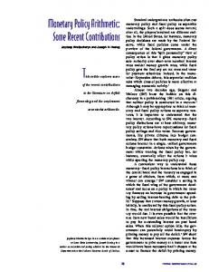
Figure 1 shows the expansion of reserves in the United States during 2008 and 2009. The solid line represents total reserves, and these grew from $45 billion in August 2008 to over $1 trillion by the last two months of 2009. Initially, most of this growth represented an increase in borrowed reserves as would be expected normally in a …nancial crisis with the central bank acting as a lender of last resort. Borrowed reserves peaked at $698 billion in November 2008 and then declined to just over $200 billion at the end of 2009. The di¤erence between total and borrowed reserves is nonborrowed reserves, and as borrowed reserves have shrunk, the Fed has expanded nonborrowed reserves so that total reserves have continued to expand. The M 1 measure of the money supply, also shown in the …gure, has risen along with total reserves. In the standard new Keynesian model, there is no independent role for monetary aggregates, given the central bank’s policy interest rate. This also implies that there is no possibility of an independent interest rate policy once monetary aggregates have been determined. This just follows from the equilibrium condition that money demand and money supply are equal. In the basic framework of a new Keynesian model, money demand is usually motivated by including real money balances in the utility function, and the …rst order condition for the representative household’s choice of money holdings states that the marginal rate of substitution between real money balances and consumption is equal to the opportunity cost of holding money, or Um (Ct ; mt ; Nt ) it = , (4) UC (Ct ; mt ; Nt ) 1 + it where C is consumption, m equals real money balances, N is labor hours,

6

i is the nominal rate of interest, and Ux denotes the marginal utility of x. If monetary policy is speci…ed in terms of the nominal interest and utility is separable in m as was assumed in (1) and (2), then it , Ct , Nt and prices are determined independently of m and (4) just residually pins down the nominal quantity of money. Quantitative easing is not a separate policy instrument. At least that is the standard analysis when the nominal interest rate is positive. At the ZLB, things may be di¤erent. When i = 0 the issue of whether an expansion in the money supply can a¤ect the real economy depends on the nature of money demand. If lim md = 1,

i!0

we have the classic case of a liquidity trap. Increases in the nominal quantity of money simply increase real balances with no e¤ect on the price level. In a liquidity trap, short-term riskless securities and money are perfect substitutes, so a substitution of money for government debt via an open market operation does not require the public to rebalance their portfolios. However, intertemporal models imply that the price level today depends on the expected future value of money. As long as nominal interest rates are expected to be positive in the future, prices in the future will depend on the future supply of money.5 An increase in the money supply now that is anticipated to be permanent will raise both expected future prices and current prices. A quantitative easing policy that leads to an expansion of the money supply at the ZLB will a¤ect the economy, as long as the rise in the money supply is expected to persist (Auerbach and Obstfeld 2005, Sellon 2003).6 5

In a basic money-in-the-utility function model, one can show that 1 = Pt

1 UC (t)

1 X i=0

i

Um (t + i) , Pt+i

where Ux (t) is short-hand for Ux (Ct ; mt ; Nt ). Even if Um (t + s) = 0 for s = 0; :::; S, the equilibrium price level is a¤ected by mt+s for s > S. See Walsh (2010, ch. 2). 6 A second aspect of an open market operation at the ZLB is that as long as nominal interest rates are expected to be positive at some point in the future, purchases of short-term government debt by the central bank alters the consolidated government’s intertemporal budget constraint. The substitution of non-interest bearing liabilities for interest-bearing liabilities lowers the present value of government revenues needs. This implies that taxes must fall, either now or in the future, to maintain budget balance. Auerbach and Obstfeld 2005 showed that these …scal e¤ects can have a signi…cant impact on nominal income at the ZLB. When prices are sticky, this rise in nominal income takes the form of an expansion in real output.

7

If, however, lim md = m > 0,

i!0

then the situation is di¤erent. The existence of a satiation level of real balances m implies that further expansions of the money quantity of money must produce increases in the price level and so changes to the current money supply can still a¤ect the economy. If interest is paid on bank reserves, then the quantity of reserves and the policy interest rate can be treated as two distinct instruments. Ignoring the distinction between money and reserves for purposes of illustration, (4) becomes Um (Ct ; mt ; Nt ) it im t = , (5) UC (Ct ; mt ; Nt ) 1 + it 7 where im t is the interest paid on money. When interest is paid on money, the Friedman distortion that arises when private agents economize on their money holdings due to a positive opportunity cost of holding money can be eliminated as long as it = im t ; the traditional Friedman rule, a de‡ation with the nominal rate equal to zero, is no longer necessary. This means that, with two instruments, monetary policy can use it to ensure a low and stable in‡ation rate and im t to ensure an e¢ cient level of money holdings. The Fed has emphasized two policy tools it can employ to tighten policy as the U.S. economy recovers: raising the interest rate paid on reserves and open market operations to reduce reserves. Payment of interest on reserves, begun in October 2008, allows the Fed to move to a channel system of interest rate control, a system successfully employed by the ECB and the central banks of Canada, New Zealand and Australia. Under such a system, the central bank establishes standing facilities for lending at a penalty over the target for the policy rate and pays interest on reserves at a rate less than the policy rate target. The interaction of reserve demand and supply in a simple channel system is illustrated in Figure 2.8 For simplicity, the …gure assumes a symmetric channel centered around the target interest rate equal to i. The upper boundary, indicated by the horizontal dashed line, is equal to i plus the discount window lending rate at the penalty rate i + p; the lower bound is the rate paid on reserves, i p. Reserve demand is the blue, downward 7 It is important to note that the interest paid on reserves must be …nanced through tax revenues and not by simply creating additional reserves. Otherwise, the opportunity cost of holding money is not altered. 8 Such a system has been analyzed by Woodford 2001 and Whitesell 2006. See also Walsh 2010, ch. 11.

8

sloping line that asymptotes at i + p and i p. Reserve supply is indicated by the vertical line. In the case illustrated, the equilibrium interbank rate is equal to the rate the central bank pays on reserves. A key aspect of a channel system is that the level of the target interest rate and the quantity of bank reserves are decoupled. The target interest rate can be increased, for example, shifting the channel upwards, without changing the quantity of reserves. Because the interest rate paid on reserves is increased in line with the target rate, the opportunity cost of holding reserves remains unchanged. Because the Fed now has the ability to pay interest on reserves, it could conceivably move to raise interest rates as the economy recovers without needing to reduce the huge expansion in reserves that has occurred over the past two years. 2.2.2

Credit easing

The Federal Reserve has also engaged in what Ben Bernanke (2009) has called credit easing. Credit easing policies are associated with changes in the composition of the central bank’s asset holdings.9 These policies have included lending to …nancial institutions, providing liquidity to speci…c credit markets, and purchasing longer-term securities. The …rst two of these categories, lending to …nancial institutions and providing liquidity, seem natural extensions of the traditional lender of last resort function of a central bank. What has di¤erentiated these policies is their extension to non-bank institutions, re‡ecting the growth in recent decades in non-bank …nance relative to bank …nance in the United States. During the past two years, the size of the Fed’s asset holdings and their composition have changed dramatically. The initial expansion of the Fed’s asset holdings occurred through its programs to extend credit and liquidity to …nancial institutions. The growth in these two categories is shown in Figure 3. After averaging $30.5 billion from January 2007 until the end of July 2007, they rose to a peak of $1,944.8 billion in December 2008. Since then, this category of asset holdings has declined signi…cantly, so that by the end of March 2010, they totaled $117.6 billion. The pattern re‡ected in Figure 3 is consistent with the behavior of a lender of last resort, providing temporary liquidity to markets during a crisis and then allowing this credit extension to shrink as markets return to more normal conditions. However, while lending to …nancial institutions and the provision of liquidity have returned to something approaching pre-crisis levels, the size of 9 Carlson, Haubrich, Cherny, and Wake…eld (2009) provide a nice discussion of the asset side of the Fed’s balance sheet.

9

the Fed’s balance sheet has not. As lending and liquidity programs have shrunk, the Fed has purchased longer-term securities representing direct obligations of Fannie Mae, Feddie Mac and Federal Home Loan Banks as well as mortgage-backed securities. This expansion in long-term security holdings is shown in Figure 4. As of the end of March 2010, the Fed held $1,284.9 billion of these securities. The e¤ectiveness of credit easing policies that alter the composition of the central bank’s asset holdings rests on the extent to which …nancial markets are segmented. The rationale for purchasing long-term securities, similar to that of “Operation Twist”in the 1960s, is to reduce the spread between long and short-term interest rates. If long-term and short-term debt are imperfect substitutes in private sector portfolios, then altering their relative supplies should move their relative yields. Central bank purchases that reduce the supply of long-term debt in private holdings would then raise their price and lower long-term yields.10 During the monetarists-Keynesian debates of the 1960s, both sides of the debate took the view that …nancial and real assets were imperfect substitutions. Both sides emphasized that shifts in portfolio composition generated by open market operations required adjustments in relative returns and asset prices to restore equilibrium. (Meltzer 1995, Tobin 1969, Goodfriend 2000, Andrés, López-Salido, and Nelson 2004). Disagreement focused on the range of assets that were potential substitutes for money holding in private portfolios. Monetarists emphasized that portfolio rebalancing could a¤ect real asset holdings, not just …nancial holdings (see Meltzer 1995). Thus, the reduction in the liquidity yield of money that occurs when its quantity is increased causes a substitute into both …nancial and real assets. Since the private sector must, ultimately, hold the larger stock of money, this attempt at rebalancing portfolios raises the prices of both …nancial and real asset, creating incentives for capital goods producers to expand production. As noted by Clouse, et. al (2003), an open market operation in longterm government debt by the central bank is equivalent to a standard open market purchase of short-term debt for money plus a purchase of long-term debt …nanced by a sale of central bank holdings of short-term government debt, in e¤ect, an operation that twists the maturity structure of privately held government debt. Whether such debt management operations are e¤ective is an empirical issue, and an issue that has, at least in the United States, long been 10 As with open market operations in standard short-term debt, changes in the composition of government debt will have …scal implications; see Auerbach and Obstfeld (2005).

10

debated. Modigliani and Sutch (1967) found little evidence that Operate Twist mattered in the 1960s, though this probably re‡ected the small scale of the operation relative to o¤setting operations by the Treasury. Prior to the current crisis, many argued that it would require extremely large open market operation in non-standard assets to have a signi…cant impact on yields (e.g., Clouse, et. al. 2003). Bernanke, Reinhart, and Sack (2004) o¤er one of the most extensive attempts to employ e¤ect studies and term structure models to determine if non-standard central bank open market operations have a¤ected yields. Their general conclusion is that shifts in relative asset supplies, or the expectations of such shifts, do a¤ect yields. However, it is not clear from their analysis whether these shifts lead to the sustained movements in relative yields that would be need to successfully stabilize real economic activity. Gagnon et. al. (2010) discuss some of the more recent evidence and conclude that announcements of the Fed’s asset purchases has lowered yields, though, as they note, using an announcement approach (as did Bernanke, Reinhart, and Sack 2004) to capture the e¤ects relies on the assumption that …nancial markets are e¢ cient in processing information. This assumption might be suspect as the rationale for credit easing policies is that …nancial markets are not operating e¢ ciently. Gagnon et. al. (2010) also provide some time series evidence on the impact on yields of the net supply of long-term debt held by the private sector. Using monthly data from 1985 until June 2008, just prior to the start of the Fed’s purchases, they …nd that an increase in the debt stock held by the public lower prices and raised yields by a statistically signi…cantly amount.11 They conclude that the size of the Fed’s purchases reduced yields by between roughly 40 and 80 basis points, depending on their empirical speci…cation. One potential problem with this estimate is that it assesses the size of the Fed’s purchases assuming that the total stock of long-term government debt is …xed. However, while the average maturity of Federal government debt held privately has fallen from 57 months at the beginning of 2008 to 49 months by September 2009, total debt (as a percent of GDP) held by the public has risen dramatically. As Figure 5 show, despite the Fed’s long term asset purchases, the stock of privately held long-term government debt has risen. the spread between the rates on 10-year and 1-year Treasury debt has not fallen, though the spread between the 1-year rate and the rate on mortgages has dipped. Thus, while the Fed purchases may have reduced 11

Their point estimates implied that an increase in longer-term debt supply equal to 1 percent of GDP (around $140 billion at 2008 GDP) would raise the 10-year term premium by between 4:4 and 6:4 basis points.

11

rates relative to the increase that might have been observed, it is less clear what the net impact on rates has been. Spiegel (2006) summarizes some of the evidence on the impact of the Bank of Japan’s purchases of long-term government bonds and quantitative easing policies that expanded bank reserves. Spiegel concludes that the two policies did lower long-term interest rates but that it is di¢ cult to determine which policy was most e¤ective. The policies may also have lowered rates by signalling the Bank of Japan’s willingness to maintain its zero interest rate policy. If purchases of long-term debt are e¤ective in stimulating aggregate demand, there remains the question of why they should be carried out by the central bank. These operations shorten the maturity structure of the Treasury’s outstanding debt. The Treasury can alter the composition of its outstanding publicly held debt; there is no reason this should be done by the central bank. Holding long-term debt on its balance sheet exposes the central bank to losses when interest rates eventually rise. Goodfriend (2000) discusses how this necessitates greater coordination between the central bank and the …scal authority and stresses the need for a Treasury guarantee against such losses. Clouse, et. al. (2003) also consider this issue. Finally, the central bank can conduct open market operations in private sector credit instruments as the Fed has done. Clouse, et. al. (2003) note that such actions would put the central bank in the position of evaluating credit risk and a¤ecting the allocation of credit across borrowers in the private sector. Relative to open market operations in government debt, the supply of private credit instruments is not exogenous; central bank purchases that raised the price of such instruments and lowered their return would in all likelihood induce an expansion of issues by the private sector. In fact, the real e¤ects of such operations would in part rest of the transference of risk from the private sector to the central bank. However, contract enforcement may be a smaller problem for central bank intermediated debt, thereby reducing borrowing limitations that would otherwise constrain private sector borrowing (see Gertler and Karadi 2009).

3

The policy framework

The policy interest rate, the rate paid on reserves, and commitments to the future path of policy rates are all likely to be important instruments of monetary policy. But what objectives should these tools be used to achieve? The consensus view leading into the …nancial crises was that best practice

12

monetary policy could be summarized as a policy of ‡exible in‡ation targeting.12 The name re‡ected the primacy of in‡ation as the ultimate objective of monetary policy; the ‡exibility re‡ected the short-run trade o¤ between in‡ation control and real economic stability that would make strict in‡ation targeting –an exclusive focus on stabilizing in‡ation –too costly to be socially desirable. Flexible in‡ation targeting is generally de…ned as a monetary policy designed to stabilize in‡ation around a low target rate and to stabilize real economic activity as measured by an output gap. In academic research, ‡exible in‡ation targeting is modeled by assuming the central bank implements policy to minimize a quadratic loss function of the form i X h i ( t+i )2 + x2t+i (6) i=0

where t is in‡ation, is the in‡ation target, and xt is the output gap. Equation (6) can represent the objectives of formal in‡ation targeters as well has those of central banks such as the Federal Reserve that emphasize the role of real objectives in addition to in‡ation. Of course, a quadratic loss function such as (6) long predates the development of in‡ation targeting. It played a key role in models of the time inconsistency of optimal monetary policy that, during the 1980s and 1990s, focused on explaining the high in‡ation rates experienced by many economies beginning in the late 1960s.13 In the more recent literature, this type of loss function is justi…ed on both positive grounds as a reasonable representation of the actual objectives of policy makers and on normative grounds as a second order approximation to the welfare of the representative agent in standard new Keynesian models (Rotemberg and Woodford 1997, Woodford 2003). In the context of the standard model, stabilizing in‡ation (actually, around a zero steady-state level) contributed to maximizing welfare because the presence of sticky prices leads, in the face of in‡ation volatility, to an ine¢ cient dispersion of relative prices. In e¤ect, in‡ation makes the price system work less e¤ectively. Prior to the crisis, in‡ation targeting (IT) was widely accepted as a successful policy framework, and recent favorable reviews of IT include Rose 12

Svensson (2002) summarized many of features of the consensus monetary policy and provided prescriptions for implementing monetary policy aimed at achieving low and stable in‡ation while also minimizing ‡uctuations in the real economy. 13 Those models assumed that the output objective in the loss function incorporated a target level for output that exceed the natural rate of output.

13

(2007) and Walsh (2009a). IT was successful in supporting low and stable in‡ation without generating the greater output volatility its critics had predicted. The …nancial crisis, though, has raised new questions about the future of in‡ation targeting. The primary concern with in‡ation targeting, even of the ‡exible variety, was that other legitimate goals of macroeconomic policy will be neglected. Initially, this concern focused on the possibility that in‡ation targeting central banks would ignore real objectives such as stabilizing the output gap (for example, see B. Friedman 2004). Part of the reluctance of the Federal Reserve to adopt in‡ation targeting could be traced to its formal dual mandate –price stability and maximum sustainable employment –and the notion that the second component of this mandate would be sacri…ced under in‡ation targeting. As surveyed in Walsh (2009a), the empirical evidence does not support this view, at least with respect to output volatility. IT countries have not experienced any cost in terms of greater real economic instability. And while the consensus view that monetary policy should only be concerned with in‡ation and output gap stability may have contributed to the …nancial crisis by ignoring …nancial distortions, this failure was not limited to IT central banks. For emerging market economies, in fact, the adoption of in‡ation targeting has been associated with improved real and in‡ation macroeconomic performance. For high income economies, the bene…ts have been, perhaps less apparent as both in‡ation targeters and non-targeters bene…ted from the Great Moderation. However, in‡ation targeting de…nitely did not contributed to an increase in real economic volatility. While it is easy to forget, the chief policy concern in 2006-2007 was the potential in‡ationary e¤ects of the dramatic increase in commodity prices. However, Rogers (2010, p. 48) concludes that “In‡ation-targeting economics appear to have done better than others in minimizing the in‡ationary impact of the 2007 surge in commodity prices...Among low-income economics, however, non-in‡ation-targeting countries experienced bigger increases in in‡ation than in‡ation-targeting economics, although their gross domestic product growth rates fell by similar amounts. Among high-income economies, in‡ation-targeting countries had a smaller growth rate decline than nonin‡ation-targeting countries and slightly less of an increase in in‡ation.”(p. 48) The recent …nancial crisis has raised new concerns about in‡ation targeting. Of course, it seems unfair to blame IT for a crisis whose origins were in the United States, as the Federal Reserve is not a formal in‡ation targeter. If one views the …nancial crisis primarily as a negative aggregate demand 14

shock causing both output and in‡ation to decline, then even a strict in‡ation targeter would respond with expansionary policies as it attempted to prevent the collapse of aggregate spending. The result that policy needs to neutralize the impact of movements in the natural real interest rate is not dependent on assuming any particular weight on real versus in‡ation goals in the central bank’s objective function. One case in which natural real rate shocks might be only partially neutralized arises if the central bank prefers to limit volatility in its policy interest rate. If it does, then the policy rate will generally be moved too little to prevent real rate shocks from a¤ecting the real economy. However, the standard argument for reducing interest rate volatility is that it re‡ects a desire by policy makers to reduce …nancial market instability. Such a motive would not support the argument that in‡ation-targeting central banks were insensitive to …nancial markets. And, just as the standard description of in‡ation targeting assumes the central bank engages in ‡exible in‡ation targeting to avoid unnecessary volatility in real output, it is also appropriate under ‡exible in‡ation targeting to ensure that achieving tighter control over in‡ation does not generate excessive …nancial instability. In fact, in‡ation targeters have fared reasonably well since the crisis began. Tables 1-3 document the experiences of 33 high income counties, of whom 10 were in‡ation targeters. Table 1 reports the average growth rate of real GDP for the 1995-2007 period, for 2008-2009, and, using the IMF forecasts, 2008-2010. While both in‡ation targeters and non-targeters have seen sharp falls in real growth, the in‡ation targeters have, as a group, done somewhat better. Table 2 reports average CPI in‡ation rates. Perhaps somewhat surprising, average in‡ation has been higher among the targeters. And while average in‡ation is expected to be higher during 2008-2010 for the IT countries than it was during 1995-2007, it is projected to be lower for the non-IT countries. At a minimum, the evidence does not seem to be that IT countries su¤er greater output declines because their central banks are too focused on controlling in‡ation. Finally, Table 3 shows the …gures for unemployment rates. There is little to di¤erentiate the IT and non-IT countries with respect to the behavior of unemployment over the crisis, though average unemployment is higher in all periods for the non-IT countries. Despite this relative success, reforms and replacements for in‡ation targeting have been proposed. I discuss three possible changes to in‡ation targeting. One would involve aiming for higher average rates of in‡ation; one would add additional objectives to the central bank’s list of goals; the 15

…nal would move to a policy of price level targeting.

3.1

Raising the in‡ation target

Prior to the crisis, a consensus existed among high income in‡ation targeters that a target within the range of 1 3 percent represented an appropriate goal for average in‡ation. This range is consistent with formal targets established by in‡ation targeting central banks (see Table 4). Developing economies normally chose higher average target in‡ation rates, though among 26 in‡ation targeters, only …ve had wider bands than 1 percent around the target (see Table 4). For example, the Bank of Korea currently has a target of 3 percent, 1 percent. Central banks that have not formally adopted in‡ation targeting also seem to have implicit targets that fall in the 1 3 percent range. For example, the Federal Reserve does not announce a formal target for the in‡ation rate, but it is reasonable to interpret the long-term in‡ation forecast of members of the Federal Open Market Committee (FOMC) as equivalent to an implicit in‡ation target. This central tendency forecast for in‡ation in the longer term measured by the price index for personal consumption expenditures ranges between 1:5 and 2 percent. The ECB has stated publicly that in‡ation should remain at or below 2 percent. If the ZLB poses a serious constraint on the ability of monetary policy to respond to economic contractions, then one change to IT would be to increase the average target for in‡ation. The lower the in‡ation target, the more likely the ZLB is encountered, a point …rst made by Summers (1991). Reifschneider and Williams (2000) estimated that the ZLB is encountered almost 10 percent of the time at a 1 percent in‡ation target, and this frequency falls as the target is raised. A higher in‡ation target would leave more room for interest rate cuts in a crisis before encountering the zero lower bound. Williams (2009) …nds that the ZLB has proven to be a hindrance to economic recovery in the aftermath of the recent …nancial crisis, concluding that “....if recent events are a harbinger of a signi…cantly more adverse macroeconomic climate than we have enjoyed over the preceding two decades, then a 2 percent steady-state in‡ation rate may be insu¢ ciently high to stop the ZLB from having signi…cant deleterious e¤ects on the macroeconomy if the central bank follows the standard Taylor rule.” (p. 3) Using the FRB/US model and a Taylor rule to represent monetary policy, Williams (2009) shows that in simulation exercises using shocks drawn from the 1968-2002 period that the nominal rate falls below 0:01 percent in 16

13 percent of the periods when the equilibrium real interest rate plus the in‡ation target equal 3 percent. Raising the in‡ation target by 2 percentage points (so the the mean nominal rate is 5 percent), reduces this probability of the ZLB to 4 percent. What matter for determining the frequency with which the ZLB is encountered are the distribution of the shocks a¤ecting the real interest rate and the target in‡ation rate. Given the real rate, a higher in‡ation target reduces the chances the ZLB will become a constraint on policy. Williams (2009) concludes that “The analysis in this paper argues that an in‡ation target of between 2 and 4 percent will, on average, be su¢ cient to avoid the ZLB causing sizable costs in terms of macroeconomic stabilization even in a much more adverse macroeconomic climate.”(p. 26) Blanchard, et al (2010) are perhaps the most prominent proponents of raising the in‡ation target, and they have argued that a 4% average rate would constitute a safer target by providing more room for interest rate cuts when the economy faces an adverse shock. While accepting that higher in‡ation is distortionary, they suggest that many of these distortions could be eliminated if tax systems were corrected to allow for higher average in‡ation. Higher in‡ation might induce more widespread wage indexation which would then hinder the ability of the economy to adjust to shocks requiring adjustment of real wages. Blanchard, et. al also recognize that we do not really know whether in‡ation expectations would be more di¢ cult to anchor if average in‡ation rates were to rise. Most of the analysis of the ZLB has been conducted using linear monetary policy rules. As Blanchard, et. al. (2010), suggest, the asymmetry introduced by the ZLB may require a non-linear reaction by central banks. As in‡ation falls, should central banks “err on the side of a more lax monetary policy, so as to minimize the likelihood of de‡ation, even if this means incurring the risk of higher in‡ation in the event of an unexpectedly strong pickup in demand”? (p. 11) While raising the average in‡ation target may reduce the constraint posed by the ZLB, higher in‡ation does have costs, and in‡ation can generate a number of distortions that reduce economic e¢ ciency and welfare. Bailey (1956) and Friedman (1969) identi…ed the ine¢ ciency that arise when nominal interest rates are positive. Since money is costless to produce, e¢ ciency requires that the private opportunity cost of holding money also be zero. If nominal interest rates are positive, private agents will ine¢ ciently economize on their money holdings. An increase in the average rate of in‡ation would increase this e¢ ciency cost. The size of the welfare cost due to this distortion of moving from 2 to 4 percent average in‡ation is likely to be small. Ireland (2009) has recently estimate the welfare cost due to reduced 17

money holdings in the United States. He …nds that, using a measure of the money stock that accounts for some of the changes due to …nancial market deregulation, the welfare cost of 2 percent in‡ation is less than 0:04 percent of income. However, higher in‡ation need not raise the opportunity cost of holding money if money pays an own return that also rises with in‡ation. If i is the market rate of interest and im is the nominal interest rate paid on money, then eliminating the Friedman distortion simply requires that i = im , not that i = 0. While there may be technical di¢ culties in paying interest on cash, many countries, including now the United States, pay interest on bank reserves. If it becomes feasible to pay explicit interest on money, then the Friedman welfare costs of moving from an average in‡ation rate of 2 percent to one of 4 percent are likely to be small. Of course, paying interest on money has …scal implications. the interest on money cannot be …nanced by printing additional money –attempting to do so rises i as in‡ation rises but fails to close the gap between i and im . Other sources of …scal revenue must be used to …nance interest on money, and this will require increases in other potentially distorting taxes. The more recent literature on wage and price stickiness has emphasized a second distortion that would be worsened by a rise in‡ation. When the adjustment of wages and prices is staggered across …rms, and is not fully indexed, higher in‡ation generates an increase in relative wage and price dispersion. Because this dispersion is not generated by any fundamental shifts in the demand or supply of individual products or labor types, economic ef…ciency is reduced. Essentially with sticky wages and prices, in‡ation makes the price system work less e¢ ciently as resources are reallocated in response to relative price and wage changes. In‡ation reduces the ability of the price system to signal shifts in demand and supply that call for a reallocate of resources. In calibrated models, this e¢ ciency loss arising from relative price dispersion is signi…cantly larger than the costs Friedman identi…ed. Thus, even if the Friedman distortion is eliminated by paying interest on money, higher in‡ation could generate signi…cant welfare costs by reducing the ability of the price system to direct resource allocation e¢ ciently. In models that derive a loss function such as that given in (6) by taking a second order approximation to the utility function of the representative agent, a failure to stabilize in‡ation around zero is more costly than allowing the output gap to ‡uctuate. For example, in the calibration of Woodford (2003), is equal to the elasticity of in‡ation with respect to marginal cost divided by the price elasticity of demand faced by individual …rms. With standard 18

values of the key parameter, this works out to a = 0:12 when in‡ation is expressed at annual rates.14 This price dispersion ine¢ ciency is related to in‡ation variability and not necessarily to the average level of in‡ation. If …rms indexed prices to the average rate of in‡ation, as is commonly assumed in many of the empirically estimated models employed for policy analysis, then a move from say 2 percent to 4 percent average in‡ation would not a¤ect the dispersion of relative prices. However, since the micro data provide no evidence of this type of indexation, an increase in the average rate of in‡ation is likely to reduce the ability of the price system to e¢ ciently guide the allocation of resources. Besides reducing the chances of hitting the ZLB, other arguments have been made in favor of higher average in‡ation. For example, one traditional argument for a bit of in‡ation is that it increases the ‡exibility of real wages if nominal wages display downward rigidity. Akerlof, Dickens, and Perry (1996) suggested that, due to the resistance to nominal wage cuts, the longrun (unemployment) Phillips curve is not vertical but has a negative slope at low rates of in‡ation. Thus, higher average in‡ation would lower the average rate of unemployment. This issues has recently been revisited by Benigno and Ricci (2010) who show how the Phillips curve ‡attens at low rates of in‡ation and shifts with changes in macro volatility. They argue that how low in‡ation should be kept can vary across countries depending on structural characteristics of the economy. If downward real wage stickiness is the problem, note that with trend productivity at 2 2:5 percent, and average in‡ation of 1 3 percent, nominal wage growth should be around 3 5:5 percent per year. This seems su¢ cient to avoid the distortions associated with any failure of wages to be ‡exible in the downward direction. In addition, the evidence on wage stickiness is mixed. Pissarides (2009) concludes that wage stickiness does not explain the volatility of unemployment, and Kudlyak (2009) …nds that the real user cost of labor is fairly cyclically sensitive. The evidence suggests that wages for new hirers display much greater ‡exibility than wages for existing workers. Thus, at the margin relevant for hiring decisions, wage stickiness may be less important. However, whenever a contraction leads …rms to reduce 14

This is based on a Calvo frequency of price adjustment of ! = 0:25 per quarter, a discount factor of = 0:99 and a demand elasticity of = 11. The formula for is =

1

(1

!)(1 !

19

! )

.

their workforce by more than can be achieved through normal turnover, the in‡exibility of nominal wages of existing workers can prevent the adjustment of real wages. A more e¤ective strategy for avoiding the ZLB would be reduce the risks of another major negative shock to aggregate demand. Better …nancial market regulation, as well as a more active response of monetary policy to emerging …nancial imbalances could lower the chances of returning to the ZLB. The permanent distortionary costs of higher average in‡ation would need to be balanced against the low probability of another negative shock of the magnitude the global economy experienced in 2008. Clouse,. et. al. (2003) note that low in‡ation at the beginning of the 1953, 1956, and 1960 recessions in the U.S. did not pose a constraint on monetary policy. Interest rates were reduced, but the ZLB was not reached. Finally, in considering whether average in‡ation targets should raised, it is important to recall that central banks have spend the past twenty…ve years striving to reduce in‡ation and to gain the credibility necessary to maintain in‡ation at low and stable rates. The stability of in‡ation expectations has been a characteristic of the recent crisis, a stability that might have been less likely during earlier periods in which the commitment of central banks to low and stable in‡ation was less clear. This credibility may be put at risk if in‡ation targets are increased.

3.2

Adding other objectives

A second issue for in‡ation targeting is whether additional objectives should be included with in‡ation and output gap stability. The theoretical rationale for ‡exible in‡ation targeting was based on models in which stabilizing the in‡ation gap and the output gap succeeded in minimizing the distortions in the economy.15 When additional distortions are present, then a policy aimed at minimizing the welfare costs of economic ‡uctuations will need to expand the list of objectives beyond the minimization of in‡ation and output gaps.16 As recent research has shown, frictions in credit and labor markets also call for the central bank to consider additional policy objectives. I will brie‡y review some of the literature in each area. 15

This is not quite right. These models generally assume a …scal subsidy is used to address the average distortion created by monopolistic competition. Consistent with that literature, I will continue to focus on the distortions that can be ameliorated by monetary policy. 16 For example, when nominal wages are sticky, optimal policy needs to consider a wage in‡ation gap as well as an in‡ation gap.

20

3.2.1

Credit frictions

The …nancial crisis has, quite understandably, generated an enormous literature examining the implications of credit frictions for monetary policy. Examples include Christiano, et. al. (2007), Cúrdia and Woodford (2008, 2009), De Fiore and Tristani (2009), Demirel (2009), Faia and Monacelli (2007), Gertler and Karadi (2009), and Gertler and Kiyotaki (2010), and the list of papers in this area continues to grow. Much of this work has built on the agency cost model of Bernanke and Gertler (1989) and Bernanke, Gertler, and Gilchrist (1999). Asymmetric information between borrowers and lenders can generate a wedge between lending rates and the opportunity cost of funds; this wedge is a¤ected by balance sheet considerations and asset prices. With asset prices and cash ‡ows moving pro-cyclically, agency costs fall in booms and rise in downturns. Thus, a recession that weakens balance sheets also increases credit spreads, amplifying the e¤ects of the original source of the cyclical movement. In normal times, therefore, balance sheet e¤ects may be an important channel through which monetary policy actions a¤ect the real economy. The role of asset prices Leading up to the crisis, there was an active debate over the appropriate role of asset prices in the conduct of monetary policy (Borio and White 2003, Cecchetti, et. al. 2000, 2002), but the consensus view was articulated by Bernanke and Gertler in 2001: “Changes in asset prices should a¤ect monetary policy only to the extent that they a¤ect the central bank’s forecast of in‡ation.”(Bernanke and Gertler 2001) Bernanke and Gertler indicated another situation in which asset prices might be relevant: if the equilibrium real interest rate were to be a¤ected by …nancial market disturbances, then the policy interest rate would need to adjust to prevent these disturbances from a¤ecting either in‡ation or the output gap.17 Consider the problem of minimizing (6), given the structure of the economy represented by (1) and (2). Optimal policy can be characterized by a targeting rule that takes the form18 t

+

(xt

xt

1)

= 0.

(7)

If monetary policy a¤ects the economy with a lag, optimal policy involves 17 18

See also Kohn 2008. This describes optimal commitment policy from the timeless perspective.

21

adjusting the policy instrument to ensure the expected value of this condition holds (Svensson and Woodford 2005), or Et

t+i

+

(xt+i

xt+i

1)

= 0.

(8)

It follows that any variable zt other than in‡ation and the output gap is relevant for optimal policy in only two circumstances. If, conditional on the past history of in‡ation and the output gap, zt Granger causes either in‡ation or the output gap, then zt can be useful in forecasting the variables that appear in the optimal targeting rule (8). Or, from (1), if, conditional on the past history of in‡ation and the output gap, zt Granger causes the natural real rate of interest, then it is relevant for setting the policy instrument consistent with (8). These conditions apply to asset prices, but they also apply to any other variable the central bank might consider responding to. The empirical research has not found consistent evidence for the value of …nancial variables in predicting in‡ation or output. Stock and Watson (2003, p. 822) conclude that “Some asset prices have been useful predictors of in‡ation and/or output growth in some countries in some periods.”Thus, while asset prices might in principle be among the macro variables that the central bank should respond to, in practice their lack of forecasting ability was viewed as rendering them largely irrelevant for monetary policy. Are asset prices only relevant if they aid forecasting? The issue of forecasting value is an empirical one. An alternative perspective is to ask whether the addition of stock prices to a simple policy rule of the Taylor variety would lead to improved outcomes as measured by in‡ation and output gap stability. That is, does responding to asset prices improve policy outcomes? The literature that has investigated this question, even using models with credit frictions of various types, has generally concluded that asset prices can safely be ignored. For example, Bernanke and Gertler (2001) evaluate policy rules in a model with …nancial frictions and …nd little value in responding to asset prices. Similarly Cúrdia and Woodford (2008) …nd that a targeting rule such as (7) that ignores credit frictions performs well. Several papers have shown that monetary policy should dampen volatility in credit spreads (e.g., Cúrdia and Woodford 2008, De Fiore and Tristani 2009). In these models, ‡uctuations in credit spreads re‡ect ine¢ ciencies that reduce social welfare. Cúrdia and Woodford assume borrowing and lending must occur through a …nancial intermediary, and real resources are 22

required to carry out this intermediation service. The credit spread ‡uctuates as a result of ine¢ cient variations in the markup of lending rates over borrowing rates. In De Fiore and Tristani (2009), credit spreads arise from agency costs and can ‡uctuate ine¢ ciently, and optimal policy involves moving interest rates inversely with shocks to the credit spread. Demirel (2009) …nds that frictions associate with monitoring costs in …nancial markets increase the weight that should be placed on stabilizing real economic activity relative to in‡ation. Although the exact channels are model dependent, ‡uctuations in credit spreads can a¤ect both aggregate demand and aggregate supply. On the demand side, they act as an ine¢ cient tax on investment; on the supply side they a¤ect …rm borrowing costs and therefore marginal costs. Thus, a rise in the credit spread reduces aggregate demand and simultaneously increases in‡ation. This suggests that the appropriate policy response to a rise in credit spreads will be uncertain. The contractionary impact on demand would call for a more expansionary policy –an interest rate reduction could o¤set partially the implicit tax on investment spending –yet the in‡ationary e¤ect on marginal costs would call for a tighter monetary policy. The basic channels of monetary policy are illustrated in Figure 8, which shows impulse responses from a VAR estimated over the 1974:1 - 2007:4 period using quarterly U.S. data. The VAR includes a measure of the output gap (log real GDP minus the log of the CBO estimate of potential GDP), in‡ation (PCE less food and energy), the funds rate, the 10 year Treasury rate (FCM10), the spread between the Baa corporate bond rate and the 10year Treasury rate, and the exchange rate (log trade-weighted real exchange rate).19 To make the …gure easier to read, the responses to output and in‡ation shocks are not shown. The standard output decline and in‡ation price puzzle phenomenon are seen in response to a funds rate shock (column 1). The rise in the funds rate leads to an increase in the long-term rate, but the spread on corporate bonds over the 10-year rate falls initially before rising. Finally, the dollar appreciates. Innovations to the credit spread variable (column 3) lead to declines in both output and in‡ation, indicating that these shocks primarily act as aggregate demand shocks. In response, the funds rate falls. Finally, an innovation to the exchange rate (an appreciation, column 4) has little e¤ect on output but does lead to a decline in in‡ation and interest rates. The impulse responses to the credit spread reported in Figure 8 suggest that shocks to the credit spread have primarily operated 19 The sample start date is determined by the availability of the exchange rate series. The end date is chosen to exclude the recent …nancial crisis.

23

as aggregate demand shocks. Therefore, a rise in spreads would call for a cut in the policy rate. Because credit spreads are directly observable and do not display trending behavior, estimating the benchmark for de…ning a credit spread gap may be a less di¢ cult problem than in the case of stock prices. If the steady state credit spread is constant, ‡uctuations in spreads may provide some re‡ection of ine¢ ciencies that monetary policy can help stabilize. However, the way policy should respond to credit spreads to stabilize real economic activity is not always so clear. For example, in work by Faia and Monacelli (2007), variants of simply Taylor rules that allow for a reaction to the price of capital (the asset price in their model) are analyzed. They …nd that strict in‡ation stabilization is optimal. However, assuming the central bank responds moderately to in‡ation (a coe¢ cient equal to 1.5) and does not respond to output (output is in the rule, not an output gap), welfare is improved if policy does respond to asset prices. But the response calls for cutting interest rates in response to a rise in asset prices. Intuitively, the reason for this response is that Faia and Monacelli assume productivity shocks are the source of ‡uctuations. In this case, …nancial frictions limit any increase in investment spending in the face of a positive productivity disturbance. This is ine¢ cient, so monetary policy can improve outcomes by reducing the interest rate. This helps move the level of investment closer to the e¢ cient level. One advantage of the analysis of Faia and Monacelli (2007) is that policy outcomes are evaluated on the basis of the implications for the welfare of the representative agent in the economy. This means that the costs of …nancial market distortions are explicitly accounted for in judging alternative policies. This is in contrast to some of the earlier work such as Bernanke and Gertler (2001) who used a loss functions such as (6) to rank policies, thereby ignoring any potential gains from responding to …nancial market distortions. Financial market segmentation A di¤erent form of …nancial friction arises in the presence of market segmentation. One type of market segmentation arises due to limited participation in …nancial markets. For example, in the typical limited participation model, households were locked into portfolio choices prior to the occurrence of any open market operations.20 Only banks and …rms continued to interact in …nancial markets when the central bank intervened. As a consequence, open market operations had distribu20

Alvarez, Atkeson, and Kehoe (2002) develop a model of endogenous market segmentation.

24

tional e¤ects as any change in the level of base money has to be absorbed by only a subset of the economy’s agents. Monetary shocks generate e¤ects on real interest rates by imposing restrictions on the ability of agents to engage in certain types of …nancial transactions. The restrictions on …nancial trading mean that cash injections via open market operations can create a wedge between the value of cash in the hands of household members shopping in the goods market and the value of cash in the …nancial market. A cash injection lowers the value of cash in the …nancial market and lowers the nominal rate of interest. Standard limited participation models assume that …rms must borrow to fund their wage bill, so the appropriate marginal cost of labor to …rms is the real wage times the gross rate of interest on loans. Thus, an interest-rate decline lowers the marginal cost of labor; at each real wage, labor demand increases. As a result, equilibrium employment and output rise. If 1 denotes the value of money in the goods market (for instance due to the assumption of a cash-in-advance constraint) and 2 denotes the value of money in the …nancial market, a standard limited participation model (see Walsh 2010, ch. 5) implies that the log-linearized expectational IS relation becomes ct = Eh ct+1

1

(it

Eh

t+1 )

1 C

(

1t

2t )

where C is steady-state consumption. This expression would, in the absence of the last term, be a standard Euler condition linking the marginal utility of consumption at t and t + 1 with the real return on the bond as in (1). But in contrast to (1), if the value of cash in the goods market di¤ers from its value in the loan market, 2t 1t 6= 0, a wedge is created between the current marginal utility of consumption and its future value adjusted for the expected real return. As a consequence, …nancial factors a¤ect current aggregate spending. Thus, with segmented …nancial markets, developments in the …nancial sector can have direct e¤ects on demand; the dichotomy between real and monetary factors that characterizes the standard new Keynesian model breaks down. Financial frictions due to agency costs and those due to market segmentation can interact. Most models have focused on frictions between lenders and …rms, but problems during the recent crisis seemed to have a¤ected the ‡ow of funds between …nancial institutions. This suggests intermediaries also have problems raising funds from other intermediaries, for example in an interbank market. Gertler and Kiyotaki (2010) show that, in the absence

25

of an agency problem in the interbank market, funds can ‡ow to banks …nancing …rms with investment opportunities from those banks without investment opportunities. Disruptions in the interbank market can a¤ect real activity, leading …nancial markets to become segmented and generate an ine¢ cient allocation of funds among intermediaries (and hence among …rms). In the face of a negative shock to the quality of capital, Gertler and Kiyotaki (2009) …nd that central bank allocation of credit to those markets with large spreads can dampen the e¤ects of the shock. This type of policy response can be likened to the Fed’s credit easing policies. Summary on …nancial frictions Most of the recent research has focused on how …nancial frictions a¤ect the transmission process of monetary policy. Fluctuations in credit spreads and borrowing constraints matter for aggregate spending, and monetary policy may be able to a¤ect them directly. Distortions in …nancial markets that generate real e¤ects of monetary policy also imply that …nancial stability may require making trade-o¤s with the goals of in‡ation stability and stability of real economic activity. While measures such as credit spreads may provide one measure of the type of inef…cient ‡uctuations that would call for a policy response, we still do not fully understand the factors that generate movements in spreads, or the degree to which these movements re‡ect ine¢ cient ‡uctuations that call for policy responses. This discussion has focused on the role of …nancial variables in nonbubble situations. A separate issue, and one actively debated during the past decade, is whether monetary policy should attempt to lean against asset price bubbles. Cecchetti, et. al (2000), Cecchetti, et. al. (2003), and Borio and White (2003) have argued that central banks should. Yet the consensus view prior to the crisis was that policy makers were limited in their ability to identify bubbles, and even if they could identify a bubble, monetary policy was too blunt an instrument to deal with this problem (Bernanke and Gertler 2001, Gertler 2003, Bernanke 2002, Kohn 2008). While monetary policy may, in general, be a blunt tool for dealing with an asset price bubble, housing investment and house prices are in fact the chief channel through which the interest rate policy of the Federal Reserve a¤ects real economic activity. The housing bubble was eventually popped by the Fed’s tighten of policy beginning in 2004. Undoubtedly, future policy makers will be more willing to risk undertaking policies to de‡ate incipient bubbles, though the di¢ culty of identifying them with certainty will always remain.

26

3.2.2

Labor market frictions

Credit frictions have not been the only frictions modern models have incorporated into frameworks for designing monetary policy. A large literature has studied the implications of two types of frictions that characterize labor markets. First, since the original work of Erceg, Henderson, and Levin (2000), it has become common, at least in empirical policy models, to incorporate nominal wage rigidities. The staggered adjustment of wages generates an ine¢ cient dispersion of relative wages whenever nominal wage in‡ation deviates from zero. Optimal policy the resulting welfare cost against the welfare costs of relative price dispersion that is generated when price in‡ation deviates from zero. If, as a result of real shocks, real wages need to adjust, the goals of price stability and of wage stability clash. Second, an alternative literature has worked to embed unemployment into DSGE models, and much of this literature has explored the consequences of labor market search frictions within the Mortensen-Pissarides model (e.g., Walsh 2005 and the survey by Galí 2010). In this class of search models, the initial employment level (the number of matches) is a critical state variable that a¤ects the dynamics of economic adjustment, and the evolution of employment depends on the incentives …rms have to create jobs and the frictions that prevent unmatched vacancies and unemployment workers from quickly matching. Ravenna and Walsh (2010) show that in a basic model with labor search frictions the welfare-consistent loss function takes the form Et

1 X

i

2 t+i

+

2 x xt+i

+

2 t+i

,

i=0

where the new term, 2t , is the squared deviation of labor market tightness (vacancies relative to unemployment) around its e¢ cient level. That is, it is appropriate to stabilize a labor market gap.21 The intuition behind the appearance of labor market objectives for policy is instructive. Recall that price in‡ation is costly because it generates an ine¢ cient dispersion of relative prices. This reduces welfare because, conditional on total consumption, it leads the economy to produce an ine¢ cient bundle of goods. Similarly, when market production is subject to frictions in matching workers and …rms, deviations of labor market tightness from its e¢ cient level lead, for 21

As Ravenna and Walsh show, of unemployment.

t

can be equivalently expressed in terms of a measure

27

a given level of utility, to an ine¢ cient combination of market production (which incurs search costs) and non-market activities (which do not incur search costs). Thus, frictions in the labor market can made labor market conditions and variables such as the unemployment rate appropriate objectives for monetary policy, though as with the output gap, it is not the level of labor market variables that should be stabilized but only their volatility around a correctly de…ned but di¢ cult to measure e¢ cient level. 3.2.3

Summary on policy objectives

Standard new Keynesian models for monetary policy emphasize the importance of price stability and lead to a speci…cation of policy objectives that is naturally characterized in terms of ‡exible in‡ation targeting. However, the only distortion amenable to monetary policy actions in the basic versions of these models arises from the presence of sticky prices, so it is not surprising that policy should o¤set this distortion by stabilizing prices. In models with multiple distortions, such as ine¢ ciencies in credit markets or in labor markets, policy makers face multiple and con‡icting objectives. Eliminating any one distortion, such as by focusing solely on price stability, may lead to suboptimal outcomes by worsening other economic distortions. Despite this, a common result in much of the literature that has focused on multiple sources of distortions is that price stability is often a close approximation to the optimal policy. For example, this is the …nding of Faia and Monacelli (2008) in a model with credit frictions and Thomas (2008) and Ravenna and Walsh (2010) in models with labor market frictions.

3.3

Price level targeting

The constraint posed by the zero lower bound on the nominal policy interest rate has led to renewed interest in price-level targeting as an alternative to IT. The arguments in favor of price level targeting take two form. First, price level targeting may have some advantages to the extent that it can lead in‡ation expectations to act as an automatic stabilizer. Second, price level targeting, by reducing errors in forecasting future prices, may reduce long-term risk and facilitate economic planning by households and …rms in a way that dominates in‡ation targeting. I will focus on the …rst of these two arguments – employing expectations as automatic stabilizers – in part because the di¤erence in forecast error variances for long-term price level forecasts under PLT and IT seems small. For example, Kahn (2009), in

28

updating estimates originally due to McCallum (1999), …nds that with a current price level set at 100 and a target in‡ation rate of 2 percent, the 95 percent con…dence interval for the price level in twenty years would be [147 157]; this represents a range of 3:2 percent around the expected price path. This seems a relative small degree of uncertainty relative to other sources of both macro and individual uncertainty faced over a twenty year period. 3.3.1

Expectations as automatic stabilizers

An advantage of price-level targeting is its ability to mimic an optimal commitment policy when the actual regime is one of discretion (Svensson 1999, Vestin 2006). This improvement occurs even though in‡ation stability is the ultimate objective of the central bank. The knowledge that prices will return to a target level in‡uences expected in‡ation in ways that help to stabilize current in‡ation when price setting behavior is forward looking.22 This role for expectations can be particularly important in a de‡ationary situation at the zero lower bound. As the actual price level falls, the gap widens between the actual price level and the path for prices implied by the target path. The more severe the de‡ation, the greater must be the subsequent in‡ation to return prices to their intended path. Thus, a credible commitment to PLT would cause expected in‡ation to rise, helping to boost nominal interest rates above the ZLB. That is, under PLT, expectations serve as an automatic stabilizer. In a basic model such as that given by (1) and (2), price-level targeting improves over discretion when an economy experiences an in‡ation shock, and PLT and IT perform equally well in the face of shifts in the equilibrium natural real rate of interest, as long as the ZLB is avoided. When the ZLB is binding, price-level targeting ensures expectations of future in‡ation move in a stabilizing fashion. In practice, most discussions of PLT combine it with a positive trend or average rate of in‡ation so that the target path is given by pTt = p0 +

T

t,

where T is the average rate of in‡ation and p0 is the initial price level. This process for the target makes pTt a trend stationary variable so that the subsequent in‡ation needed after a deviation of prices below the target path rises with T . A positive trend to the price path strengthens the way 22 Not surprising, therefore, Walsh (2003) found that price level targeting performed less satisfactorily in a discretionary environment when the in‡ation process displays inertia.

29

expectations act as an automatic stabilizer after de‡ationary shocks since with the target path rising over time, the gap between it and the actual price level, such a de‡ation occur, grows over time and ampli…es the rise in expected in‡ation (if the path is credible). The e¤ect on in‡ation expectations of adopting PLT will depend on when it is adopted and how quickly the public expects deviations from target to be eliminated. Figure 6 shows the price level in the U.S., measured by the PCE chained index together with hypothetical 1:5 percent and 2:0 percent paths. These rates correspond to the upper and lower ranges of the longerrun in‡ation forecasts of the FOMC members. One set of paths begins in January 2007, the other in January 2008. As the …gure shows, when price level targeting is adopted and what the average rate of in‡ation is matter for the way in‡ation expectations are likely to be a¤ected. If the Fed had adopted price level targeting with a 2:0 percent drift in January 2007, the movement of the PCE index above the target path would have called for a tighter monetary policy throughout 2008 and would have generated expectations of de‡ation over this period. Thus, it is not evident that adopting PLT would have contributed a stabilizing in‡uence, nor would it have generated increases in expected in‡ation that might have reduced real interest rates at the ZLB. The story is somewhat more supportive of a contributing role for PLT if it had been adopted in January 2008. The PCE index has fallen persistently below even the 1:5 percent price path in this case, suggesting that credible price level targeting might have raised expected in‡ation. The impact on in‡ation expectations of deviations from a price level target depend on how quickly the public anticipates that the price level will return to its target path. Figure 7 shows hypothetical paths for expected in‡ation under a price-level targeting regime in the U.S. based on two different start dates, January 2007 and January 2008, under the assumption that the public expects prices to return to target within four quarters. In the top panel, the price level is assumed to be measured by the PCE, and the target path rises at a 1:75 percent annual rate, the mid-point of the FOMC’s central tendency. The bottom panel uses the PCE excluding food and energy. Also shown in each panel is a line at 1:75 percent, corresponding to in‡ation expectations anchored under an in‡ation targeting regime. In the top panel, the paths for expectations under price level targeting for both start dates fall below 1:75 percent for part of the period, particularly in the …rst half of 2008 when expectations actually turn negative based on the January 2007 start date. Because in‡ation rose above the assumed 1:75 percent target in 2007, a price-level targeting policy would have required a de‡ation 30

by early 2008. Of course, incorporating a higher trend in‡ation rate into the price path would shift the paths for expected in‡ation up. However, this would not change the conclusion that establishing a price-level target in early 2007 would have initially produced a fall in expected in‡ation. Expectations would have moved in the wrong direction, exacerbating the ZLB problem.23 Because actually in‡ation in the U.S. has remained relatively stable, falling from October 2008 through January 2009 but then returning to levels similar to those seen in 2006 and 2007, the path of the core PCE excluding food and energy shown in the bottom panel of Figure 7 has not diverged much from the hypothetical target paths. As a consequence, expectations would have remained close to the level of the in‡ation target. The hypothetical paths in the …gure assume complete credibility of the price-level targeting regime. Just as the adoption of in‡ation targeting did not produce immediate credibility, it is likely that any switch to price-level targeting would involve gradual learning on the part of the public before the regime gained the level of credibility now enjoyed by in‡ation targeting. Kryvtsov, Shukayev, and Ueberfeldt (2008) show that the gains from imperfectly credible price-level targeting in a calibrated model are fairly small, and the gains may not be su¢ cient to dominant in‡ation targeting if credibility is obtained slowly.24 However, repeating this exercise using the Bank of Canada’s policy model ToTEM, Cateau, et. al. (2008) found the ultimate gains from price-level targeting to be more signi…cant.25 In general, the work on price-level targeting may understate its advantages for two reasons. First, the analysis based on model simulations often ignores the ZLB, and a credible regime of price-level targeting has advantages over in‡ation targeting at the ZLB. Second, models typically ignore an important …nancial frictions –nominal debt contracts. While nominal interest rates can adjust to compensate for average in‡ation expected over the duration of a contract, PLT, by increasing the predictability of the future price level, can reduce risk premiums associated with nominal contracts. In a DSGE model estimated using Canadian data and including agency costs 23 Of course, this analysis ignores the fact that the price level might have evolved di¤erently during 2007 and 2008 if the Federal Reserve had adopted price-level targeting. 24 They ignore the ZLB in their analysis. 25 Battini and Yates (2003) consider what they describe as hybrid in‡ation and pricelevel targeting. The central bank is assigned an objective that combines both in‡ation and the price level, and optimal trade-o¤ frontiers are mapped. They argue that much of the bene…t of price-level targeting is obtained when only a small weight is placed on the price level in the objective that guides the design of policy. See also Billi (2008).

31

and nominally denominated debt, Dib, Mendicino, and Zhang (2008) …nd that PLT reduces the volatility of the real interest rate. This helps reduce distortions associated with nominal contracts.26 To summarize, PLT has advantages over in‡ation targeting by stabilizing the real interest rate, which can reduce …nancial frictions, and by ensuring in‡ation expectations act to help automatically stabilize in‡ation. This improves the trade-o¤ between output and in‡ation stabilization. 3.3.2

Should central banks adopt PLT at the ZLB?

PLT can contribute to better macroeconomic stability at the ZLB. Given this advantage over IT, should central banks adopt PLT? Several points are relevant for evaluating this question. First, PLT does not eliminate the possibility of a liquidity trap. For example, if monetary policy is implemented using a Taylor rule in which in‡ation deviations from target are replaced by price level deviations from target, an expectational-driven liquidity trap is still possible.27 However, when the economy is pushed into a liquidity trap as a result of a fall in the equilibrium real interest rate, PLT ensures expectations move in a manner that helps to stabilize the economy. Despite this, there are several reasons for questioning the e¢ cacy of adopting price-level targeting when an economy is at the ZLB. First, the stabilizing adjustment of expectations arises only if the public understands the implications of price-level targeting and believes the central bank is committed to this new policy. The experience with in‡ation targeting was that credibility followed experience and the gain in anchoring expectations was not something that was achieved immediately. Gaining credibility for PLT in the midst of a liquidity trap may be particularly challenging. The optimal time-varying price-level target path would be di¢ cult to communicate to the public. This is a serious limitation since PLT’s advantages arise from the way it allows expectations to be steered. While past commitment to a price 26

They also provide references to the related literature investigating price-level targeting with nominal contracts. 27 For example, if it = rtn + (pt p ), then the Fisher equation implies it = rtn + Et

t+1

= rtn + (pt

p ),

so Et pt+1 = (1 + ) pt

p .

For any > 0, pt = p is the unique solution, but there exists de‡ationary solutions beginning at any p0 < p such that i ! 0.

32

level target might aid in avoiding a ZLB or mitigating the impact of a ZLB situation, adopting a new, untested targeting regime while in a crisis seems inadvisable. In addition, at the ZLB, commitment to a price level target would, to the extent to which it was successful in generating expectations of future in‡ation, lead to a rise in long-term nominal interest rates. This rise in long-term rates may easily lead some to question the central bank’s commitment to economic expansion. Second, the impact on expectations depends importantly on the speed with which the public expects the central bank to regain the target path. This may be hard for the public to forecast since there would be no past experience to draw upon. Similarly, it may be di¢ cult for the central bank to assess the impact of the regime change on the public’s expectations. If expectations are for an extended recession, the public may doubt whether the target path will be achieved very quickly. This would reduce the e¤ect PLT would have in raising in‡ation expectations. Third, there is the question of which price index to target. Given the volatility of headline in‡ation, targeting the headline price index might generate destabilizing movements in expectations, as Figure 7 illustrated. Many critics of in‡ation targeting in open economies point to the problem of de…ning targets in terms of headline in‡ation. A depreciation then requires the central bank to contact domestic output to reduce in‡ation in domestic goods prices. This potential problem is even more severe with price-level targeting. Finally, commitment to a price path that involves future in‡ation is time inconsistent. Recall that the price-level target is a means of implementing the optimal commitment policy, and this policy is itself time inconsistent. Once the economy recovers from the ZLB, the optimal policy is not to create the in‡ation required to restore the price level to the promised target path. Optimal commitment means doing what you had previously promised to do, even if it is not the optimal thing to do at the moment. Many central banks have committed to in‡ation targeting. They have developed credibility by delivering low and stable in‡ation. The optimal strategy at the ZLB is to change the policy regime to one of price level targeting, and of course to promise never to change the policy framework again. Changing the policy regime in a crisis is exactly what discretion would call for.

33

4

Conclusions

In the face of multiple distortions, multiple instruments are necessary, and central banks have added to the set of tools that they can employ. While many of the actions taken during the crisis, such as private sector asset purchases or debt management operations designed to a¤ect the maturity composition of government debt, are essentially …scal operations and not likely to play a role in normal times, the payment of interest on reserves, the use of channel systems, and the separation of quantitative policies and market interest rate policies is likely to remain. The e¤ectiveness of unconventional policies such as credit easing depend on the extent to which assets are imperfect substitutes or …nancial markets are segmented. These are both aspects of …nancial markets that we do not yet fully understand. Clearly the next-generation models will incorporate credit frictions, but in the models developed to date, these frictions often do not seem to generate big di¤erences in the transmission mechanism. The sources of …nancial shocks and how best to respond to them is still an open issue on which no consensus has developed. The same is true of labor market frictions, whether arising from sticky nominal wages or from search and matching frictions. As Chari, Kehoe, and McGratten (2009) have noted with respect to the standard new Keynesian model, we need to know the sources of shocks if we are to determine whether they call for a policy response. Central banks typically argue that interest rate policy is too blunt an instrument to deal with …nancial stability and asset price bubbles and that these problems are best dealt with through well designed and implemented regulatory policies. However, even in the presence of adequate …nancial sector regulation, imperfect information and the resulting moral hazard and adverse selection problems in …nancial markets remain a source of distortions that a¤ect the appropriate objective of monetary policy. Flexible in‡ation target seems to have worked well during the crisis, but the constraints associated with the zero lower bound on nominal interest rates has led to proposals to raise average in‡ation targets. When macro volatility is at the levels seen during the Great Moderation, occurrences of the ZLB may be su¢ ciently rare that raising average in‡ation is unnecessary. But if macroeconomic shocks are likely to be larger in the future, the bene…ts of higher average in‡ation increase, though these must be balanced against the costs of higher in‡ation. Price level targeting is a viable alternative to in‡ation targeting and may lead in‡ation expectations to move in a stabilizing fashion, particularly in helping to avoid the ZLB. However, the date PLT is adopted, the choice of price index, the underlying average 34

trend in‡ation rate, and the speed with which price level deviations from the target path are expected to be reversed are all important for determining whether PLT would be a desirable policy regime.

References [1] Adams, K. and R. M. Billi,. 2006. “Optimal Monetary Policy under Commitment with a Zero Bound on Nominal Interest Rates,” Journal of Money, Credit, and Banking 39(7): 1877-1905. [2] Adams, K. and R. M. Billi. 2007. “Discretionary Monetary Policy and the Zero Lower Bound on Nominal Interest Rates.”Journal of Monetary Economics 54: 728-752. [3] Akerlof, G. A., W. R. Dickens, and G. L. Perry. 1996. “The Macroeconomics of Low In‡ation,”Brookings Papers on Economic Activity, The Brookings Institution, vol. 27, pages 1-76. [4] Alvarez, F., A. Atkeson, and P. J., Kehoe, “Money, Interest Rates, and Exchange Rates with Endogenously Segmented Markets,”Journal of Political Economy 2002, vol. 110 (1), 73-112. [5] Andrés, D. López-Salido, and E. Nelson. 2004. “Tobin’s Imperfect Asset Substitution in General Equilibrium.” Journal of Money, Credit, and Banking 36(4), Aug. 665-90. [6] Auerbach, A. J. and M. Obstfeld. 2005. “The Case for Open-Market Purchases in a Liquidity Trap.”American Economic Review 95(1): 110137. [7] Bailey, M. J., “The Welfare Costs of In‡ationary Finance,” Journal of Political Economy, 64(2), Apr. 1956, 93-110. [8] Battini, N. and A. Yates. 2003. “Hybrid In‡ation and Price-Level Targeting.” Journal of Money, Credit, and Banking. 35(3):283-300. [9] Benigno, P. and L. A. Ricci, “The In‡ation-Output Trade-O¤ with Downward Wage Rigidities,” NBER Working Paper 15762, Feb. 2010. [10] Bernanke, B. S. 2002. “Asset-Price ‘Bubbles’ and Monetary Policy,” Remarks before the New York Chapter of the National Association for Business Economists, New York, NY, Oct. 15.

35

[11] Bernanke, B. S. 2009. [12] Bernanke, B. S. and M. Gertler. 1989. “Agency Costs, Net Worth, and Business Fluctuations,” American Economic Review, 79(1): 14-31. [13] Bernanke, B. S. and M. Gertler. 2001. “How Should Central Bankers Respond to Asset Prices?”American Economic Review Papers and Proceedings 91(2): 253-257. [14] Bernanke, B. S., M. Gertler, and S. Gilchrist. 1999. “The Financial Accelerator in a Quantitative Business Cycle Framework,”in J. B. Taylor and M. Woodford (eds.), Handbook of Macroeconomics, Vol. 1C, Amsterdam: Elsevier North-Holland, 1341-1393. [15] Bernanke, B. S., V. R. Reinhart, and B. P. Sack. 2004. “Monetary Policy Alternatives at the Zero Bound: An Empirical Assessment.”Brookings Papers on Economic Activity. [16] Billi, R. M., “Price-Level Targeting and Risk Management in a LowIn‡ation Economy,” Federal Reserve Bank of Kansas City, Nov. 2008. [17] Blanchard, O., G. delil’Aricca, and P. Mauro, “Rethinking Macroeconomic Policy,” IMF Sta¤ Position Note, SPN/10/13, Feb. 12, 2010. [18] Board of Governors of the Federal Reserve System. 2009. Monetary Policy Report to the Congress. July. [19] Borio, C. and W. R. White. 2003. “Whither Monetary and Financial Stability? The Implications of Evolving Policy Regimes.” Monetary Policy and Uncertainty: Adapting to a Changing Economy. A Symposium Sponsored by the Federal Reserve Bank of Kansas City. 131-211. [20] Carlson, J., J. G. Haubrich, K. Cherny, and S. Wake…eld. 2009. “Credit Easing: A Policy for a time of Financial Crisis,” Economic Trends, Federal Reserve Bank of Cleveland. Feb. 11, 2009. [21] Cateau, G., O. Kryvstov, M. Shukayev, and A. Ueberfeldt. 2008. “Adopting Price-Level Targeting under Imperfect Credibility in ToTEM.” Bank of Canada Working Paper 2009-17. [22] Cecchetti, S. G. 2008. “Crisis and Response: The Federal Reserve and the Financial Crisis of 2007-2008.” NBER Working Paper 14134.

36

[23] Cecchetti, S. G., H. Genberg, J. Lipsky, and S. Wadhwani. 2000. “Asset Prices and Central Bank Policy.” Geneva Reports on the World Economy, No. 2. [24] Cecchetti, S. G., H. Genberg, and S. Wadhwani. 2002. “Asset Prices in a Flexible In‡ation Targeting Framework.” NBER Working Paper No. W8970. [25] Chari, V. V., P. J. Kehoe and E. R. McGrattan. 2009. “New Keynesian Models: Not Yet Useful for Policy Analysis,” American Economic Journal Macroeconomics, 1(1): 242-266. [26] Christiano, L., R. Motto, and M. Rostagno, “Financial Factors in Business Cycles,” Nov. 2007. [27] Clarida, R., J. Galí, and M. Gertler. 1999. “The Science of Monetary Policy: A New Keynesian Perspective,” Journal of Economic Perspectives 37(4): 1661-1707. [28] Clouse, J., D. Henderson, A. Orphanides, D. H. Small and P. A. Tinsley. 2003. “Monetary Policy When the Nominal Short-Term Interest Rate is Zero.” Topics in Macroeconomics 3(1): Article 12. [29] Cúrdia, V. and M. Woodford. 2008. “Credit Frictions and Optimal Monetary Policy,” Discussion Papers 0809-02, Columbia University. [30] Cúrdia, V. and M. Woodford. 2008. “Conventional and Unconventional Monetary Policy,” Nov. 2009. [31] De Fiore, F. and O. Tristani. 2009. “Optimal Monetary Policy in a Model of the Credit Channel.” March. [32] Del Negro, M., G. Eggertsson, A. Ferrero, and N. Kiyotaki. 2010. “The Great Escape? A Quantitative Evaluation of the Fed’s non-Standard Policies,” Feb. 2010. [33] Demirel, U. D. 2009. “Optimal Monetary Policy in a Financially Fragile Economy.” The B.E. Journal of Macroeconomics: Contributions 9(1): Article 15. [34] Dib, A., C. Mendicino, and Y. Zhang. 2008. “Price-Level Targeting in a Small Open Economy with Financial Frictions: Welfare Analysis.” Bank of Canada Working Paper 2008-40.

37

[35] Eggertsson, G. B. and M. Woodford. 2003. “The Zero Bound on Interest Rates and Optimal Monetary Policy,” Brookings Papers on Economic Activity, 1, 139-211. [36] Erceg, C. J., D. Henderson, and A. T. Levin, “Optimal Monetary Policy with Staggered Wage and Price Contracts,” Journal of Monetary Economics, 46(2), Oct. 2000, 281-313. [37] Faia, E. and T. Monacelli. 2007. “Optimal Interest rate Rules, Asset Prices, and Credit Frictions,”Journal of Economic Dynamics and Control. 31: 3228-3254. [38] Friedman, B. M. 2004. “Why the Federal Reserve Should Not Adopt In‡ation Targeting,” International Finance, 7(1): 129-136.53. [39] Friedman, M., “The Optimum Quantity of Money,”in his The Optimum Quantity of Money and Other Essays, Chicago: Aldine Publishing Co., 1969. [40] Gagnon, J., M. Raskin, J. Remarche, and B. Sack, “Large-Scale Asset Pruchases by the Federal Reserve: Did They Work,” Federal Reserve Board, Sta¤ Report no. 441, March 2010. [41] Galí, J. 2010. “Monetary Policy and Unemployment,” NBER Working Paper 15871, forthcoming, Handbook of Monetary Economics. [42] Galí, J. and M. Gertler. 2007. “Macroeconomic Modeling for Monetary Policy Evaluation,” Journal of Economic Perspectives, 21(4): 25-46. [43] Gertler, M. 2003, “Commentary: Whither Monetary and Financial Stability? The Implications of Evolving Policy Regimes.” Monetary Policy and Uncertainty: Adapting to a Changing Economy. A Symposium Sponsored by the Federal Reserve Bank of Kansas City. 213-223. [44] Gertler, M. and P. Karadi. 2009. “A Model of Unconventional Monetary Policy.” [45] Gertler, M. and N. Kiyotaki. 2009. “Financial Intermediation and Credit Policy in Business Cycle Analysis.” [46] Goodfriend, M. 2000. “Overcoming the Zero Bound on Interest Rate Policy.”Journal of Money, Credit, and Banking 32(4), pt. 2: 1007-1035. [47] Goodfriend, M. 2007. “How the World Achieved Consensus on Monetary Policy,” Journal of Economic Perspectives, 21(4): 47-68. 38

[48] Gruen, D.. M. Plumb, and A. Stone, “How Should Monetary Policy Respond to Asset-Price Bubbles?”International Journal of Central Banking Dec. 2005, 1(3): 1-31. [49] Hutchison, M. M., T. Ito, and F. Westermann. 2006. “The Great Japanese Stagnation: Lessons for Industrial Countries.” Japan’s Great Stagnation: Financial and Monetary Policy Lessons for Advanced Industrial Countries. M. M. Hutchison and F. Westermann (eds.) The MIT Press. [50] Ireland, P. N., “On the Welfare Cost of In‡ation and the Recent Behavior of Money Demand,” American Economics Review 99(3), June 2009, 1040-1052. [51] Ito, T. 2004. “In‡ation Targeting and Japan: Why Has the Bank of Japan Not Adopted In‡ation Targeting? NBER Working Paper 10818. [52] Kahn, George A., 2009. “Beyond In‡ation Targeting: Should Central Banks Target the Price Level?” Federal Reserve bank of Kansas City Economic Review. [53] Kohn, D. L. 2008. “Monetary Policy and Asset Prices Revisited,” Speech to the Cato Institute’s 26th Annual Monetary Policy Conference, Washington, D.C., Nov. 19. [54] Krugman, P. R. 1998. “It’s Baaack: Japan’s Slump and the Return of the Liquidity Trap,” Brookings Papers on Economic Activity. 2: 137205. [55] Kryvstov, O., M. Shukayev, and A. Ueberfeldt. 2008. “Adopting PriceLevel Targeting under Imperfect Credibility.”Bank of Canada Working Paper 2008-37. [56] Kudlyak, M. 2009. “The Cyclicality of the User Cost of Labor with Search and Matching,” FRB of Richmond WP No. 09-12. [57] Levin, A., D. López-Salido, E. Nelson, and T. Yun. 2009. “Limitations on the E ectiveness of Forward Guidance at the Zero Lower Bound,” International Journal of Central Banking forthcoming. [58] McCallum, B. T. 1999. “Issues in the Design of Monetary Policy Rules,” in J. B. Taylor and M. Woodford, Handbook of Macroeconomics, Amsterdam: Elseview Science B. V., vol. 1C, 1483-1530. 39

[59] McCallum, B. T. 2000. “Theoretical Analysis Regarding a Zero Lower Bound on Nominal Interest Rates.” Journal of Money, Credit, and Banking, 32(4): 870-904. [60] Meltzer, A. H. 1995. “Monetary Credit and (Other) Transmission Processes: A Monetarist Perspective.” Journal of Economic Perspectives 9:49-72. [61] Mishkin, F. S.. 2009. “Is Monetary Policy E¤ective during Financial Crises?” American Economic Review, 99(2), May, 573-577. [62] Modigliani, Franco, and Richard Sutch. 1967. “Debt Management and the Term Structure of Interest Rates: An Empirical Analysis of Recent Experience.” Journal of Political Economy 75: 569-89. [63] Nakov, A. 2008. “Optimal and Simple Monetary Policy Rules with Zero Floor on the Nominal Interest Rate,” International Journal of Central Banking, 4(2): 73-128. [64] Nishiyama, S.-I. 2009. “Monetary Policy Lag, Zero Lower Bound, and In‡ation Targeting,” Bank of Canada Working Paper 2009-2. [65] Pissarides, Christopher A., “The Unemployment Volatility Puzzle: Is Wage Stickiness the Answer?,” Econometrica, 2009, 77(5): 1339-1369. [66] Ravenna, F. and C. E. Walsh. 2010. “Welfare-based optimal monetary policy with unemployment and sticky prices: A linear-quadratic framework.” [67] Reifschneider, D. and J. Williams. 2000. “Three Lessons for Monetary Policy in a Low In‡ation Era.”Journal of Money, Credit, and Banking, 32(4): 936–66. [68] Reinhart, C. M. and K. S. Rogo¤, This Time is Di¤ erent: Eight Centuries of Financial Folly, Princeton, N.J.: Princeton University Press, 2009. [69] Roger, S., “In‡ation Targeting Turns 20,” Finance and Development, March 2010, 46-49. [70] Rose A. K. 2007. “A Stable International Monetary System Emerges: Bretton Woods, Reversed,” Journal of International Money and Finance.

40

[71] Rotemberg, J. J. and M. Woodford, “An Optimizing-Based Econometric Model for the Evaluation of Monetary Policy,” NBER Macroeconomic Annual 1997, Cambridge, MA: MIT Press, 297-346. [72] Sellon, G. H. Jr. 2003. “Monetary Policy and the Zero Bound: Policy Options When Short-Term Rates Reach Zero.” Federal Reserve Bank of Kansas City Economic Review Fourth Quarter: 5-43. [73] Spiegel, M. M. 2006. “Did Quantitative Easing by the Bank of Japan ‘Work’?” Economic Letter, Federal Reserve Bank of San Francisco, 2006-28, Oct. 20. [74] Stock, J. H. and M. W. Watson. 2003. “Forecasting Output and In‡ation: The Role of Asset Prices.” Journal of Economic Literature 41: 788-829. [75] Summers, L.. 1991. “Panel Discussion: How Should Long-Term Monetary Policy Be Determined?” Journal of Money, Credit, and Banking 23(3, Pt 2): 625-631. [76] Svensson, L. E.O. 1999. “Price Level Targeting vs. In‡ation Targeting,” Journal of Money, Credit, and Banking, 31: 277-295. [77] Svensson, L. E. O. 2001. “The Zero Bound in an Open Economy: A Foolproof Way of Escaping from a Liquidity Trap,”Monetary and Economic Studies, 19, S-1, 277-312. [78] Svensson, L. E. O. 2002. “Monetary Policy and Real Stabilization,” Federal Reserve Bank of Kansas City Jackson Hole Symposium, Rethinking Stabilization Policy, 261-312. [79] Svensson, L. E. O. 2003., “Escaping from a Liquidity Trap and De‡ation: The Foolproof Way and Others,” Journal of Economic Perspectives, 17, 145-166. [80] Svensson, L. E. O. and M. Woodford. 2005. “Implementing Optimal Policy through In‡ation-Forecast Targeting,” in Bernanke, B. S., and M. Woodford, eds., The In‡ation-Targeting Debate, Chicago, University of Chicago Press, 19-83. [81] Thomas, C. 2008. “Search and Matching Frictions and Optimal Monetary Policy,” Journal of Monetary Economics 55, 936-956

41

[82] Tobin, J. 1969. “A General Equilibrium Approach to Monetary Theory.” Journal of Money, Credit, and Banking 1: 15-29. [83] Vestin, D. 2006. “Price-Level Targeting versus In‡ation Targeting,” Journal of Monetary Economics 53(7): 1361-1376. [84] Walsh, C. E., “Speed Limit Policies: The Output Gap and Optimal Monetary Policy,”American Economic Review, 93(1), March 2003, 265278. [85] Walsh, Carl E., “Labor Market Search, Sticky Prices, and Interest Rate Policies,” Review of Economic Dynamics, 8(4), Oct. 2005, 829-849. [86] Walsh, C. E. 2009a. “In‡ation Targeting: What Have We Learned,”the John Kuszczak Memorial Lecture, the Bank of Canada, International Finance, 12(2): 195–233. [87] Walsh, C. E., 2009b. “Using monetary policy to stabilize economic activity,” Federal Reserve Bank of Kansas City Financial Stability and Macroeconomic Policy¸2009 Jackson Hole Symposium, forthcoming. [88] Walsh, C. E. 2010. Monetary Theory and Policy, 3rd ed., The MIT Press. [89] Whitesell W. 2006. “Interest Rate Corridors and Reserves.”Journal of Monetary Economics 53(6): 1177-1195. [90] Williams, John C., “Heeding Daedalus: Optimal In‡ation and the Zero Lower Bound,” Brookings Papers on Economic Activity 2009. [91] Wolman, A. 2005. “Real Implications of the Zero Bound on Nominal Interest Rates,”Journal of Money, Credit, and Banking 37(2): 274-296. [92] Woodford, M. 2001.“Monetary Policy in the Information Economy,” Federal Reserve Bank of Kansas City Jackson Hole Symposium. 297370. [93] Woodford, M. 2003. Money, Interest, and Prices, Princeton: Princeton University Press.

42

Table 1: Real GDP: Growth Rate All IT NIT 1995-2007 3:60 3:64 3:38 2008-2009 1:08 0:65 1:27 2008-2010 0:35 0:06 0:53 Change to 2009 4:54 4:29 4:64 Change to 2010 3:81 3:57 3:91 Source: IMF World Economic Outlook, March 2010 Projected Table 2: In‡ation: Average Consumer Prices All IT NIT 1995-2007 2:54 2:82 2:42 2008-2009 2:56 3:90 1:97 2008-2010 2:16 3:25 1:68 Change to 2009 0:012 1:08 0:45 Change to 2010 0:39 0:43 0:74 Source: IMF World Economic Outlook, March 2010 Projected Table 3: Unemployment Rate All IT NIT 1995-2007 6:53 5:85 6:82 2008-2009 6:30 5:63 6:59 2008-2010 6:98 6:33 7:27 Change to 2009 0:23 0:22 0:24 Change to 2010 0:46 0:48 0:44 Source: IMF World Economic Outlook, March 2010 Projected

43

New Zealand Canada UK Sweden Australia Czech Rep. Israel Poland Brazil Chile Colombia South Africa Thailand Korea Mexico Iceland Norway Hungary Peru Phillipines Guatemala Indonesia Romania Turkey Serbia Ghana

Table 4: In‡ation Targeters Year 2009 In‡ation Midpoint 1990 0:8 2 1991 0:3 2 1992 2:2 2 1993 0:3 2 1993 1:9 2:5 1997 1:0 3 1997 3:3 2 1998 3:8 2:5 1999 4:9 4:5 1999 1:5 3 1999 4:2 3 2000 7:1 4:5 2000 0:9 1:75 2001 2:8 3 2001 5:3 3 2001 12:0 2:5 2001 2:2 2:5 2001 4:2 3 2002 2:9 2 2002 1:6 4:5 2005 1:8 5 2005 4:6 5 2005 5:6 3:5 2006 6:3 6:5 2006 7:8 6 2007 19:3 14:5

Width 2 2 2 2 1 2 2 2 4 2 2 3 2:5 2 2 3 2 2 2 2 2 2 2 2 4 2

+/No Yes Yes Yes No Yes Yes Yes Yes Yes No No No Yes Yes Yes Yes Yes Yes Yes Yes No Yes Yes No Yes

Source: Scott Roger, “In‡ation targeting turns 20,” Finance and Development, March 2010, 46-49. The column indicates whether the the central bank speci…es a target rate with a symmetric band around the mid-point.

44

1200

1700

TOTAL BORROWED EXCESS M1

1650

1000

1600 800 1550 600 1500 400 1450 200

1400

0

1350 2007

2008

2009

Figure 1: Total, borrowed, excess reserves (right scale) and M1 (left scale) in the U.S. (billions of dollars)

45

0.04 0.035 id =i +p Interest rate

0.03 0.025 0.02 0.015 0.01

i r =i - p

0.005 0 -2.5

-2

-1.5

-1

-0.5 0 Reservebalances

0.5

1

1.5

2

2.5

Figure 2: Interest rate control under a channel system

x 10

5

18 16 14

billions of $

12 10 8 6 4 2 0

01/01/08

01/01/09

01/01/10

Figure 3: Unconventional policies: lending to …nancial institutions (dark blue) and liquidity provision (light blue)

46

x 10

5

18 16 14

billions of $

12 10 8 6 4 2 0

01/01/08

01/01/09

01/01/10

Figure 4: Unconventional policies: lending to …nancial institutions (dark blue), liquidity provision (light blue), and purchases of long-term assets (green) 30 25

5

PRIV_LONG FED_LONG SPREAD_1_10YR MORTSPREAD

4

20

3

15

2

10

1

5

0

0

-1 2007

2008

2009

Figure 5: Privately held Federal government debt with maturity greater than one year and Federal Reserve long-term asset purchases, both expressed as a percent of GDP. Also shown are the spreads between the yields on 1-year and 10-year Federal government debt and 30-year mortgage rate (right axis).

47

112 111 110 109 108 107 106 105 104 103 01/01/07

01/01/08

01/01/09

01/01/10

Figure 6: The PCE index and hypothetical price cones beginning January 2007 and January 2008. Lower paths correspond to 1.5% in‡ation, the upper paths to 2.0% in‡ation. 4 3 2 1 0 -1 -2 -3

IT EXP2007JC EXP2008JC

2007

2008

2009

2008

2009

4 3 2 1 0 -1 -2 -3

IT EXP2007JCXFE EXP2008JCXFE

2007

Figure 7: Expected in‡ation when prices are expected to return to the target path in four quarters with a 1:75% in‡ation rate price path. Paths are shown for PLT beginning Jan. 2007 (dotted, exp2007) and Jan. 2008 (exp2008). Top panel: PCE. Bottom panel: PCE less food and energy.

48

FFED OUTPUT

FCM10 0.4

0.4

0.2

0.2

0.2

0.0

0.0

0.0

0.0

-0.2

-0.2

5

10

15

0.3

15

-0.6 0

5

10

15

0.3

0.2

0.1 -0.0

-0.1

-0.1

-0.2

10

15

5

10

15

5

10

15

1.2 1.0

1.2 1.0

1.2 1.0

0.8 0.6 0.4

0.8 0.6 0.4

0.8 0.6 0.4

0.8 0.6 0.4

0.2 0.0 -0.2 -0.4 -0.6 0

5

10

15

0.2 0.0 -0.2 -0.4 -0.6 0

5

10

15

5

10

15

0.50

0.50

0.50

0.25

0.25

0.25

0.25

0.00

0.00

0.00

0.00

-0.25

-0.25

-0.25

-0.25

-0.50

-0.50

-0.50

-0.50

5

10

15

0

5

10

15

0

5

10

15

0.25

0.25

0.25

0.25

0.20

0.20

0.20

0.20

0.15

0.15

0.15

0.15

0.10

0.10

0.10

0.10

0.05

0.05

0.05

0.05

0.00

0.00

-0.05

0.00

-0.05

-0.10 5

10

15

5

10

15

5

10

15

0.030

0.030

0.030

0.030

0.025

0.025

0.025

0.020

0.020

0.020

0.020

0.015

0.015

0.015

0.015

0.010

0.010

0.005

0.010

0.005

0.000

5

FFED

10

15

5

FCM10

10

15

5

10

15

0

5

10

15

10

15

0.000 -0.005

-0.010 0

0

0.005

0.000 -0.005

-0.010 0

15

0.010

0.005

0.000 -0.005

-0.010

10

-0.15 0

0.025

-0.005

5

-0.10

-0.15 0

0

-0.05

-0.10

-0.15 0

15

0.00

-0.05

-0.10

-0.15

10

0.2 0.0 -0.2 -0.4 -0.6 0

0.50

0

5

-0.4 0

1.2 1.0

0.2 0.0 -0.2 -0.4 -0.6

0

-0.3

-0.4 0

15

-0.2

-0.3

-0.4 5

10

-0.1

-0.2

-0.3 0

5

0.2

0.1 -0.0

-0.4

0 0.3

0.2

0.1 -0.0

-0.3

Responses of

10

0.1

-0.2

EXCH

5

-0.0 -0.1

SPREAD

-0.4

-0.6 0

0.3

0.2

-0.2

-0.4

-0.6 0

FCM10

-0.2

-0.4

-0.6

FFED

EXCH

0.4

0.2

-0.4

INFLATION

SPREAD

0.4

-0.010 0

5

SPREAD

10

15

0

5

EXCH

Figure 8: Impulse responses from a VAR estimated for the U.S., 1974:12007:4. See text for details.

49