to solve an instance, as well as the number of backtracks, up to two orders ... below the current node and backtracks to a higher level in the search tree. If.
Improved Branch and Bound Algorithms for Max-2-SAT and Weighted Max-2-SAT ? Jordi Planes Department of Computer Science, Universitat de Lleida (Spain)
Abstract. We present novel branch and bound algorithms for solving Max-SAT and weighted Max-SAT, and provide experimental evidence that outperform the algorithm of Borchers & Furman on Max-2-SAT and weighted Max-2-SAT instances. Our algorithms decrease the time needed to solve an instance, as well as the number of backtracks, up to two orders of magnitude.
1
Introduction
In recent years we have seen an increasing interest in propositional satisfiability (SAT) that has led to the development of fast and sophisticated complete SAT solvers like Chaff [11] and Satz [8], which are based on the well-known DavisPutnam-Logemann-Loveland (DPLL) procedure [3]. Given a Boolean CNF formula φ, such algorithms determine whether there is a truth assignment that satisfies φ. Unfortunately, they are not able to solve two well-known satisfiability optimization problems: Max-SAT and weighted Max-SAT. Given a Boolean CNF formula φ, Max-SAT consists of finding a truth assignment that maximizes the number of satisfied clauses in φ. Given a Boolean CNF formula φ, where each clause has a weight, weighted Max-SAT consists of finding a truth assignment that maximizes the sum of the weights of the satisfied clauses in φ. When all the clauses have at most two literal per clause (weighted) Max-SAT is called (weighted) Max-2-SAT. To our best knowledge, there are only two exact algorithms for Max-SAT that are variants of the DPLL procedure. One is due to Wallace & Freuder [13] and the other is due to Borchers & Furmann [1]. Both are depth-first branch and bound algorithms, and were developed independently. The former was implemented in Lisp, while the latter was implemented in C and is publicly available. There are other exact algorithms for Max-SAT, but based on mathematical programming techniques [2, 4, 7]. In this paper we first describe novel branch and bound algorithms for solving Max-SAT and weighted Max-SAT that we have designed and implemented. They are variants of the algorithm of Borchers & Furmanm that incorporate more powerful lower bound calculations and variable selection heuristics. We then report on an experimental investigation we have conducted in order to evaluate ?
This Research was partially supported by the project CICYT TIC2001-1577-C03-03 funded by the Spanish Ministerio de Ciencia y Tecnolog´ıa.
our algorithms on Max-2-SAT and weighted Max-2-SAT instances. The results obtained provide experimental evidence that our algorithms outperform the algorithm of Borchers & Furman on randomly generated Max-2-SAT and weighted Max-2-SAT instances. Our approach decreases the time needed to solve an instance, as well as the number of backtracks, up to two orders of magnitude.
2
Branch and Bound for Max-SAT
The space of all possible assignments for a CNF formula φ can be represented as a search tree, where internal nodes represent partial assignments and leaf nodes represent complete assignments. A branch and bound algorithm for Max-SAT explores the search tree in a depth-first manner. At each node, the algorithm compares the number of clauses unsatisfied by the best complete assignment found so far —called upper bound (U B)— with the number of clauses unsatisfied by the current partial assignment (unsat) plus an underestimation of the number of clauses that become unsatisfied if we extend the current partial assignment into a complete assignment (underestimation). The sum unsat + underestimation is called lower bound (LB). Obviously, if U B ≤ LB, a better assignment cannot be found from this point in search. In that case, the algorithm prunes the subtree below the current node and backtracks to a higher level in the search tree. If U B > LB, it extends the current partial assignment by instantiating one more variable; which leads to create two branches from the current branch: the left branch corresponds to instantiate the new variable to false, and the right branch corresponds to instantiate the new variable to true. In that case, the formula associated with the left (right) branch is obtained from the formula of the current node by deleting all the clauses containing the variable ¬p (p) and removing all the occurrences of the variable p (¬p); i.e., the algorithm applies the one-literal rule [9]. The solution to Max-SAT is the value that U B takes after exploring the entire search tree. Borchers & Furmann [1] designed and implemented a branch and bound solver for Max-SAT that incorporates two quite significant improvements: – Before starting to explore the search tree, they obtain an upper bound on the number of unsatisfied clauses in an optimal solution using the local search procedure GSAT [12]. That improvement allows them to solve instances up to seven times faster than when they do not perform that preprocessing [1]. – When branching is done, branch and bound algorithms for Max-SAT apply the one-literal rule (simplifying with the branching literal) instead of applying unit propagation as in the DPLL-style solvers for SAT.1 If unit propagation is applied at each node, the algorithm can return a non-optimal solution. However, when the difference between the lower bound and the upper bound is one, unit propagation can be safely applied, because otherwise by fixing to false any literal of any unit clause we reach the upper bound. Borchers & Furmann perform unit propagation in that case. 1
By unit propagation we mean the repeated application of the one-literal rule until a saturation state is reached.
Our branch and bound algorithms are variants of the algorithm of Borchers & Furmann that incorporate the above improvements. Besides such improvements, there are two factors that have a dramatic impact on the performance of any branch and bound algorithm: the quality of the lower bound, and the heuristic used to select the next variable that has to be instantiated. We consider two lower bounds: – LB1 = unsat. Note that that the number of clauses unsatisfied by the current partial assignment coincides with the number of empty clauses that contains the formula associated with the current partial assignment. That elementary lower bound that does not incorporate underestimation is used by Borchers & Furmann. P – LB2 = unsat + p∈φ0 min(ic(p), ic(¬p)), where φ0 is the formula associated with the current partial assignment, and ic(p) (ic(¬p)) —inconsistency count of p (¬p)— is the number of clauses that become unsatisfied if the current partial assignment is extended by fixing p (¬p) to true (false). Note that ic(p) (ic(¬p)) coincides with the number of unit clauses of φ0 that contain ¬p (p). If for each variable we count the number of positive and negative literals in unit clauses, we can know the number of unit clauses that will not be satisfied if the variable is instantiated to true or false. Obviously, the total number of unsatisfied clauses resulting from either instantiation of the variable must be greater than or equal to the minimum count. Moreover, the counts for different variables are independent, since they refer to different unit clauses. Hence, by summing the minimum count for all variables in unit clauses and adding this sum to the number of empty clauses, we calculate a lower bound for the number of unsatisfied clauses given the current assignment. Such a lower bound was considered in [13]. And we consider three variable selection heuristics: – MOMS: selects a variable among those that appear more often in clauses of minimum size. That is the heuristic of Borchers & Furmann. – Jeroslow-Wang (JW) [6, 5]: given a formula φ, for each literal L of φ the following function is defined: X 2−|C| J(L) = L∈C∈φ
where |C| is the length of clause C. JW selects a variable p of φ among those that maximize J(p) + J(¬p). – Weighted Clause Length (WCL): let φ be a formula, let unit-clauses(L) be the number of occurrences of literal L in unit clauses of φ, let binary-clauses(L) be the number of occurrences of literal L in binary clauses of φ, let w1 , w2 be natural numbers, and let W CL(L) = w1 × unit-clauses(L) + w2 × binary-clauses(L).
WCL selects a variable p of φ among those that maximize W CL(p) + W CL(¬p). We set w1 = 1 and w2 = 3 in our experiments. Such settings were determined experimentally. We get several branch and bound algorithms by combining the above lower bounds and heuristics: LB1+MOMS, LB1+JW, LB1+WCL, LB2+MOMS, LB2+JW and LB2+WCL. LB1+MOMS corresponds to the algorithm of Borchers & Furmann. LB2+MOMS incorporates the lower bound of [13] into the algorithm of Borchers & Furmann. LB2+JW is like LB2+MOMS but uses the Jeroslow-Wang rule as variable selection heuristic. LB2+WCL is like LB2+MOMS but uses the Weighted Clause Length heuristic. LB2+MOMS and LB2+JW are two of our novel branch and bound algorithms for Max-SAT. We have implemented them by modifying the publicly available code of Borchers & Furmann. We do not consider LB1+JW because its performance is much worse than the performance of LB2+JW. For the same reason, we have not considered LB1+WCL . Input: max-sat(φ, ub) : A Boolean CNF formula φ and an upper bound ub 1: if φ = ∅ or φ only contains empty clauses then 2: return empty-clauses(φ) 3: end if 4: if lower-bound(φ) = ub − 1 then 5: φ ← unit-propagation(φ) 6: end if 7: if lower-bound(φ) ≥ ub then 8: return ∞ 9: end if 10: p ← select-variable(φ) 11: ub ← min(ub, max-sat(φ¬p , ub)) 12: return min(ub, max-sat(φp , ub)) Output: The maximum number of clauses of φ that can be satisfied Fig. 1. Branch and Bound for Max-SAT
Figure 1 shows the pseudo-code of the skeleton of the exact algorithms for Max-SAT we consider here: LB1+MOMS, LB2+MOMS, LB2+JW and LB2+WCL. We use the following notation: – empty-clauses(φ) is a function that returns the number of empty clauses in the formula φ. – lower-bound(φ) is the sum of the empty clauses of φ plus an underestimation of the number of unsatisfied clauses in the formula obtained from φ by removing its empty clauses. In our case, LB1 or LB2. – ub is an upper bound of the number of unsatisfied clauses in an optimal solution. We assume that the input value is that obtained with GSAT. – select-variable(φ) is a function that returns a variable of φ following an heuristic; in our case, MOMS, JW or WCL.
– φp (φ¬p ) is the formula obtained by applying the one-literal rule to φ using the literal p (¬p). We have also developed improved versions of LB2+MOMS, LB2+JW and LB2+WCL, which we refer to as LB2-I+MOMS, LB2-I+JW and LB2-I+WCL. In such versions, we check if we can fix the truth value of any free variable before branching. This amounts to introduce the following code after line 9: for all literal l in φ do if ic(l) > ic(¬l) and lower-bound(φ) + (ic(l) − ic(¬l)) ≥ ub then φ ← φ¬l end if end for As we show in the next section, this technique improves considerably the performance of our algorithms.
3
Experimental Results
We conducted an experimental investigation in order to compare the performance of LB1+MOMS, LB2+MOMS, LB2+JW and LB2+WCL, as well as their improved versions. In our first experiment, we solved the same instances that were used by Borchers & Furmann in [1]. They are randomly generated Max-2-SAT and weighted Max-2-SAT instances that differ in the ratio of number of clauses to number of variables. instance unsat LB1+MOMS LB2+MOMS LB2-I+MOMS LB2+JW LB2-I+JW LB2+WCL LB2-I+WCL 50 2sat 100 4 0.03 0.04 0.03 0.05 0.40 0.11 0.11 50 2sat 150 8 0.09 0.11 0.09 0.08 0.60 0.07 0.06 50 2sat 200 16 6.21 4.06 2.46 1.92 0.79 1.41 0.58 50 2sat 250 22 36 7.22 4.64 1.51 0.76 0.87 0.38 50 2sat 300 32 526 37 25 23 11 17 7.07 50 2sat 350 41 7,593 186 115 66 32 30 14 50 2sat 400 45 3,313 79 52 22 12 11 6.58 100 2sat 200 5 0.17 0.23 0.24 0.66 0.36 800 803 100 2sat 300 15 720 1,059 795 165 54 249 71 100 2sat 400 29 > 36hrs > 36hrs > 36hrs 11,602 4,619 4,547 1,525 150 2sat 300 4 0.25 0.29 0.34 4.52 1.75 > 36hrs > 36hrs Table 1. Experimental results for Borchers & Furmann’s Max-2-SAT instances. Time in seconds.
Table 1 shows the results for those random Max-2-SAT instances that can be solved in less than 36 hours by at least one of the algorithms. For each instance, we give the optimal number of unsatisfied clauses and the seconds needed to solve the instance on a 2GHz Pentium IV with 512 Mb of RAM. In the name of the instance are indicated first the number of variables, then the type of
instance unsat LB1+MOMS LB2+MOMS LB2-I+MOMS LB2-I+JW LB2+WCL LB2-I+WCL 50 2sat 100 16 0.05 0.03 0.04 0.04 0.04 0.03 50 2sat 150 34 0.06 0.04 0.04 0.04 0.09 0.05 50 2sat 200 69 0.70 0.37 0.24 0.12 0.15 0.09 50 2sat 250 96 7.10 2.28 1.38 0.62 1.25 0.61 50 2sat 300 132 27.06 4.14 2.70 0.87 1.03 0.55 50 2sat 350 211 1,278 81 54 19 20 8.88 50 2sat 400 211 635 23 16 6.40 8.42 4.69 50 2sat 450 257 2,045 39 27 5.71 3.46 2.51 50 2sat 500 318 6,113 79 53 29 24 14.43 100 2sat 200 7 0.13 0.08 0.08 0.07 0.07 0.08 100 2sat 300 67 103 75 16 15 194 18 100 2sat 400 119 36,481 13,381 2,647 2,568 34,360 4,693 100 2sat 500 241 > 36hrs > 36hrs > 36hrs > 36hrs > 36hrs 91,742 100 2sat 600 266 > 36hrs > 36hrs > 36hrs > 36hrs > 36hrs 70,350 150 2sat 300 24 0.54 0.37 0.35 1.04 861 17 150 2sat 450 9 8,282 5,323 3,012 4,502 37,451 15,188 Table 2. Experimental results for Borchers & Furmann’s weighted Max-2-SAT instances. Time in seconds.
10000
10000 1000 time (log scale)
time (log scale)
LB1+MOMS LB2+MOMS LB2+JW 1000 LB2+WCL 100 10 1 0.1 0.01 100
LB1+MOMS LB2+MOMS LB2+JW LB2+WCL
100 10 1 0.1
150
200
250
number of clauses
300
350
0.01 100
150
200
250
300
350
number of clauses
Fig. 2. Experimental results for 50-variable Max-2-SAT instances. Left plot: mean time. Right plot: median time. Time in seconds.
time (log scale)
100
1000
LB1+MOMS LB2-I+MOMS LB2-I+JW LB2-I+WCL
100 time (log scale)
1000
10 1 0.1 0.01 100
LB1+MOMS LB2-I+MOMS LB2-I+JW LB2-I+WCL
10 1 0.1
150
200 250 number of clauses
300
350
0.01 100
150
200 250 number of clauses
300
350
Fig. 3. Experimental results for 50-variable weighted Max-2-SAT instances. Left plot: mean time. Right plot: median time. Time in seconds.
instance, and finally the number of clauses. Observe that our algorithms outperform LB1+MOMS up to two orders of magnitude. As greater is the number of unsatisfied clauses in the optimal solution, the behaviour of our algorithms is better. Also observe that LB2-I+MOMS, LB2-I+JW and LB2-I+WCL outperform considerably LB2+MOMS, LB2+JW and LB2+WCL. Table 2 is like Table 1 but for weighted Max-2-SAT instances. Again we clearly see that our algorithms provide large performance improvements, which are due to the quality of the lower bounds and variable selection heuristics used. In our second experiment, we generated sets of random Max-2-SAT and random weighted Max-2-SAT instances with 50 variables and a different number of clauses. Such instances were generated using the method described in [10]. For Max-2-SAT, we generated sets for 100, 150, 200 and 250 clauses, where each set had 100 instances. For weighted Max-2-SAT, we generated sets for 100, 150, 200, 250, 300 and 350 clauses, where each set had 100 instances. The results of solving such instances with LB1+MOMS, LB2-I+MOMS, LB2-I+JW and LB2-I+WCL are shown in Figure 2 (Max-2-SAT instances) and Figure 3 (weighted Max-2SAT instances). Along the horizontal axis is the number of clauses, and along the vertical axis is the mean and median time (in seconds) needed to solve an instance of a set. Notice that we use a log scale to represent run-time. Clearly, our algorithms outperform LB1+MOMS. It is worth to note that LB2-I+WCL has the best scaling behaviour on both random Max-2-SAT and random weighted Max-2-SAT instances. As future work, we plan to experiment with other heuristics, define better lower bounds, and incorporate into our algorithms advanced data structures like those defined for SAT solvers in the last years.
References 1. B. Borchers and J. Furman. A two-phase exact algorithm for MAX-SAT and weighted MAX-SAT problems. Journal of Combinatorial Optimization, 2:299–306,
1999. 2. J. Cheriyan, W. Cunningham, L. Tun¸cel, and Y. Wang. A linear programming and rounding approach to MAX-2-SAT. In D. Johnson and M. Trick, editors, Cliques, Coloring and Satisfiability, volume 26, pages 395–414. 1996. 3. M. Davis, G. Logemann, and D. Loveland. A machine program for theoremproving. Communications of the ACM, 5:394–397, 1962. 4. E. de Klerk and J. P. Warners. Semidefinite programming approaches for MAX-2SAT and MAX-3-SAT: computational perspectives. Technical report, Delft, The Netherlands, 1998. 5. J. N. Hooker and V. Vinay. Branching rules for satisfiability. Journal of Automated Reasoning, 15:359–383, 1995. 6. R. G. Jeroslow and J. Wang. Solving propositional satisfiability problems. Annals of Mathematics and Artificial Intelligence, 1:167–187, 1990. 7. S. Joy, J. Mitchell, and B. Borchers. A branch and cut algorithm for max-sat and weighted max-sat. In DIMACS Workshop on Satisfiability: Theory and Applications, 1996. 8. C. M. Li and Anbulagan. Heuristics based on unit propagation for satisfiability problems. In Proceedings of the International Joint Conference on Artificial Intelligence, IJCAI’97, Nagoya, Japan, pages 366–371. Morgan Kaufmann, 1997. 9. D. W. Loveland. Automated Theorem Proving. A Logical Basis, volume 6 of Fundamental Studies in Computer Science. North-Holland, 1978. 10. D. Mitchell, B. Selman, and H. Levesque. Hard and easy distributions of SAT problems. In Proceedings of the 10th National Conference on Artificial Intelligence, AAAI’92, San Jose/CA, USA, pages 459–465. AAAI Press, 1992. 11. M. Moskewicz, C. Madigan, Y. Zhao, L. Zhang, and S. Malik. Chaff: Engineering an efficient sat solver. In 39th Design Automation Conference, 2001. 12. B. Selman, H. Levesque, and D. Mitchell. A new method for solving hard satisfiability problems. In Proceedings of the 10th National Conference on Artificial Intelligence, AAAI’92, San Jose/CA, USA, pages 440–446. AAAI Press, 1992. 13. R. Wallace and E. Freuder. Comparative studies of constraint satisfaction and Davis-Putnam algorithms for maximum satisfiability problems. In D. Johnson and M. Trick, editors, Cliques, Coloring and Satisfiability, volume 26, pages 587–615. 1996.