IMPROVED CORRELATION DIMENSION CALCULATION

International Journal of Bifurcation and Chaos, Vol. 11, No. 7 (2001) 1865–1880 c World Scientific Publishing Company

IMPROVED CORRELATION DIMENSION CALCULATION J. C. SPROTT Department of Physics, University of Wisconsin, Madison, WI 53706, USA G. ROWLANDS Department of Physics, University of Warwick, Coventry CV47AL, England Received August 23, 2000; Revised October 12, 2000 For many chaotic systems, accurate calculation of the correlation dimension from measured data is difficult because of very slow convergence as the scale size is reduced. This problem is often caused by the highly nonuniform measure on the attractor. This paper proposes a method for collecting data at large scales and extrapolating to the limit of zero scale. The result is a vastly reduced required number of data points for a given accuracy in the measured dimension. The method is illustrated in detail for one-dimensional maps and then applied to more complicated maps and flows. Values are given for the correlation dimension of many standard chaotic systems.

1. Introduction The most widely used tool for detecting chaos in experimental data is calculation of the correlation dimension using the method of Grassberger and Procaccia [1983a, 1983b]. The idea is to construct a correlation integral C(r) equal to the probability that two arbitrary points on the orbit in state space are closer together than r. This is usually done by calculating the separation between every pair of N data points and sorting them into bins of width ∆r proportional to r. The correlation dimension is given by D2 = d log(C)/d log(r) in the limit ∆r → 0, r → 0 and N → ∞. These limits are inherently incompatible for a finite data set, and for many attractors the computed value of D2 converges very slowly. In the Grassberger–Procaccia [1983a] paper, examples (with N = 1.5 × 104 ) are shown only for the H´enon map and Lorenz model, and it turns out that these cases are exceptional in their rapid convergence. In their longer paper, Grassberger and Procaccia [1983b] address some of

the problems of slow convergence and propose a solution of embedding the data in a higher dimension. This suggestion is helpful, but it does not cure the problem. Because of this difficulty, the literature is devoid of credible numerical calculations of the correlation dimension for most model chaotic systems, including the logistic map, the R¨ ossler attractor, and the Chirikov map. For the same reason, spuriously low dimensions have often been reported for experimental data. In this paper we describe a method for measuring the correlation integral at finite r and extrapolating to the limit of r = 0. One product of this work is improved accuracy in the measured correlation dimension of several standard chaotic systems. Throughout, the convergence difficulties experienced in the numerics are illustrated by analytic results obtained using special cases. The proposed method is based on identifying critical points of the measure that are shown to control the dimension. In the examples discussed in detail, the

1865

1866 J. C. Sprott & G. Rowlands

critical points are relatively easy to identify, but the method is applicable to more general maps and flows.

2. Theory 2.1. One-dimensional maps To study and identify the critical points in the measure and hence the convergence of the correlation dimension, we consider in some detail the onedimensional case for a variety of maps. The correlation integral C(r) is given in terms of an invariant measure P (x) by ZZ

C(r) =

P (x)P (x0 )Θ(r − |x − x0 |)dxdx0

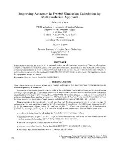
Fig. 1.

Shapes of general symmetric maps for various α.

(1) equation) the measure is

where Θ is the Heaviside function and the integrals are over the whole space of the mapping. We take the measure to satisfy the Frobenius–Perron equation (see, e.g. [Rowlands, 1990]) in the form P (x2 ) P (x1 ) + 0 + ··· P (x) = 0 |f (x1 )| |f (x2 )|

(2)

= df /dx is its where f (x) denotes the map and first derivative. Here xi are the preimages of x such that x = f (xi ). We initially restrict our attention to simple maps that have just two preimages, and in particular to maps of the form (3)

where α is a free parameter in the range 1/2 to ∞. Maps with α < 1/2 do not have chaotic solutions. The shapes of f (x) for different α are shown in Fig. 1. In particular, the case α = 2 is the wellknown logistic map [May, 1976], and α = 1 is the tent map. Each case maps the interval [0, 1] onto itself and has a maximum of f = 1 at x = 1/2. The generalization to other maps will be made after the general concepts have been illuminated. It is convenient to introduce I(r) given by dC I(r) = dr

(4)

P (x)P (x + r)dx .

1−r

dx x(x + r)(1 − x)(1 − x − r)

p

0

(7) which can be integrated analytically to give I(r) = 4P02 K(k) where K is the complete elliptic√integral of the first kind and the argument is k = 1 − r 2 . In particular, for r → 0, we have I(r) = 4P02 [2 ln 2 − ln r + O(r 2 ln r)] .

(8)

This indicates a logarithmic singularity, which we will see is a feature common to all one-dimensional maps having a single simple maximum. Using the above expansion for I(r), we find Z

r

I(r)dr

C(r) = 0

= 4P02 [(2 ln 2 + 1)r − r ln r + O(r 3 ln r)]

C(r) = ar + br ln r + O(r 3 ln r)

1−r

I(r) = 2

I(r) = 2P02

which we write in the more general form

in which case we can use Eq. (1) to obtain Z

(6)

where P0 is a normalization constant equal to 1/π. Substitution of this form into Eq. (4) gives Z

f0

f (x) = 1 − |2x − 1|α

P0 P (x) = p x(1 − x)

(5)

0

To proceed further, we use the well-known result [Rowlands, 1990] that for α = 2 (the logistic

(9)

from which it follows that 

p = ln C(r) = p + q + ln q +

a b



+ O(r 2 q) (10)

Improved Correlation Dimension Calculation 1867

where q = ln r. In the numerical evaluation of p or C(r) we can restrict the range to r  1, while |q| is order unity. In this case, terms of order r 2 q and higher can be neglected, and p can be written as 

p(q) = p + q + ln q +

a b



(11)

where p and a/b are constants which for the above case take the values p = ln(4P02 ) and a/b = −(2 ln 2 + 1) ' −2.386. A local correlation dimension ν(r) can now be defined such that ν(r) =

dp 1 r dC = =1+ a C dr dq q+ b

(12)

while the correlation dimension D2 is the q → −∞ (r → 0) limit of ν(r), which goes to 1 for the logistic map as expected. √ The above analysis illustrates that the 1/ x singularity in the measure P (x) causes ν(r) to converge logarithmically with r, making numerical evaluation of the dimension difficult. To show the ubiquitous nature of this behavior, consider the general logistic equation f (x) = Ax(1 − x). In this case, the Frobenius–Perron equation takes the form P (x) =

P (x1 ) + P (x2 ) A|1 − 2x1 |

(13)

p

 

P

(14)

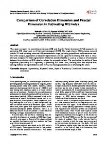
With finite P (1/2), the maximum point x = 1/2 maps to a square root singularity at x = A/4. Further mapping produces additional singularities. Figure 2 shows a typical measure with these singularities in the logistic map for A = 3.8. If we now assume that for small enough r these singularities are separated, we can write I(r) =

XZ i

xi+L

xi

g(x, r)dx (x − xi )(x − xi + r)

p

and L is much greater than r, reflecting the fact that the singularities are well separated on a scale compared to r. The case where this is no longer a reasonable assumption as for the measure on a fractal is considered later. In the small-r limit, we can evaluate the above integral by expanding g(x, r) in a Taylor series in x and r to obtain I(r) =

" X

#

g(xi , r = 0) ln r + O(r)

(16)

i

with x1,2 = (1 ± 1 − 4x/A)/2. If we now consider x ' A/4 so that both x1 and x2 are close to 1/2, the Frobenius–Perron equation gives 1 2 P (x) ∼ p . 1 − 4x/A

Fig. 2. Probability density for the logistic map with A = 3.8.

(15)

where g(x, r) is some unknown but smooth function of x and r, xi is the position of the ith singularity,

from which we can calculate C(r) and p(r). Most importantly, one finds that p(r), neglecting terms involving r explicitly, is a function of the general form given by Eq. (11) but where now p and a/b are unknown quantities of order unity. Thus the singular nature studied explicitly for the logistic map with A = 4 is expected for other values of A. Furthermore, when translated into an equation for the local correlation dimension, the same slow logarithmic convergence is expected. This latter property follows immediately from the nature of the map near its maximum. Given that the maximum of the map controls the convergence, it is important to study examples where the shape is different. A simple example is the tent map (α = 1). In this case the Frobenius– Perron equation reduces to P (x) =

P (x1 ) + P (x2 ) 2

where x1 = x/2 and x2 = 1 − x/2. An obvious solution is P (x) = 1 in the interval 0 ≤ x ≤ 1.

1868 J. C. Sprott & G. Rowlands

With the substitution x = r(1 − cosh θ)/2, Eq. (21) reduces to

Substituting this into Eq. (4) gives I(r) = 2(1 − r) C(r) = 2r − r

r I = ( )1−2β 2

2

and p(r) = p + q + ln(1 − r/2) .

(17)

Now there is no singularity, and ν(r) converges to unity as powers of r, not q. The case α = 1/2 can also be studied analytically. The Frobenius–Perron equation [Eq. (2)] for maps of the form of Eq. (3) reduces to 1 P (x) = 2α



2 1−x

β

[P (x1 ) + P (−x1 )]

(18)

where x = 2x − 1 = 1 − 2|x1 |α , x1 > 0 and β = 1 − 1/α. For α = 1/2 (or β = −1), we have

4P02 3

(19)

!

+ q + ln(1 + 3r/4) .

Again the convergence is through r, not q, and the dimension is unity. For other values of α, it has not been possible to find an analytic expression for the measure P (x). To obtain the form for ν(r), we proceed by studying the form of the singularities in P (x). This is readily found from Eq. (18) by considering x1 → 0, in which case for x ≈ 1, we obtain P (x) ≈ P0 /(1 − x)β .

(20)

Although we do not know the form for P (x) except near these critical points in the evaluation of I(r) as defined by Eq. (5), it is only these points that can give anything other than simple powers of r in I(r). Thus the major contribution to I(r) will be proportional to an integral of the form Z

I= 0

L

dx . [x(x + r)]β

sinh

(22)

(θ)

I = Ar 1−2β + B + O(r) where A and B are constants. Using this form to calculate C(r) and hence p(r), we find 

2q 2(1 − β)B 2β−1 + ln 1 + r p(r) = p0 + α A 2q 2(1 − β)B 2β−1 . + r α A 

where P0 is determined by a normalization condition. This form gives I(r) = 2(2P0 )2 (1/3 + r/2) so that p(r) = ln

0

dθ 2β−1



(23)

This corresponds to

A solution to this is simply P (x) = P0 (1 − x)

θ

where coshθ = 1 + 2L/r. For 2β > 1 (or α > 2), the integral can be divided into a part with limits 0 to ∞ and another with limits θ to ∞. In the latter we can express the sinh θ term in exponentials and evaluate the integral. In this way we obtain

≈ p0 +

1 P (x) = (1 − x)[P (x1 ) + P (−x1 )] . 2

Z

(21)



B 2β−1 r A  ν(r) =  2B 2β−1 α 1+ r αA 2 1+

(24)

where terms of order r have been neglected. The correlation dimension is now 2/α, but the convergence is no longer logarithmic in q and depends on a fractional power of r. Thus we can expect a faster convergence than for the logistic equation in any numerical scheme used to calculate this dimension. This prediction is borne out by the numerical experiments described below. For 0 < 2β < 1 (or 1 < α < 2) we have to proceed a little differently since the integral over θ from zero to infinity is infinite. We first differentiate with respect to r to give dI = −β dr

Z 0

L

dx . [x(x + r)]β (x + r)

This integral can now be evaluated the same way that I(r) was evaluated for β > 1 to give I(r) = Ar1−2β + B . Now since 2β < 1, the major contribution comes from B, but otherwise proceeding as above, we have C(r) = Br +Ar 2/α

Improved Correlation Dimension Calculation 1869

where A = αA/2, giving A p = p0 + q + ln 1 + r 2/α−1 B

!

(25)

and 2 A 2/α−1 r αB . (26) ν(r) = A 2/α−1 1+ r B Thus for α > 2 the dimension is 2/α, and for α ≤ 2 the dimension is unity. This prediction is confirmed by numerical results discussed later. Equation (18) for the measure P (x) has been solved numerically. First a function ψ(x) is introduced to take out the singular behavior and defined such that ψ(x) . (27) P (x) = (1 − x2 )β 1+

Then ψ(x) satisfies the equation ψ(x) =



1− R(x) =

(28)

2/α

1−x 2 2(1 + x)

.

(29)

R(x) is not singular at x + 1 = 0 and in fact is a monotonic function of x varying from 1/α at x = −1 to 1/4 at x = 1. Thus we expect ψ(x) to be a smooth, almost constant function. This equation has been solved by iteration, and the results fit well to a form with ψ varying slowly with x. In fact, for both α = 1 and α = 2, ψ(x) is strictly constant. The above form for ψ(x) when substituted into Eq. (27) gives a form for P (x) consistent with the singular behavior of P (x) derived directly from the Frobenius–Perron equation. Using this form for P (x) gives Z

I(r) = P02

0

1−r

2.2. Decoupled maps We have shown for a range of one-dimensional maps how the singularities in the measure, traced back to the behavior of the map in the vicinity of its maximum, determine the correlation dimension D2 and its asymptotic variation ν(r). Unfortunately, far less is known about the form of the measure in higher dimensions. In this section we consider two simple 2-D cases that can be treated to some extent analytically. One can still define a correlation function in a form similar to Eq. (1), namely ZZZZ

C(r) =

P (x, y)P (x0 , y 0 )Θ

· (r − |x − x0 | − |y − y 0 |)dxdx0 dydy 0 . (31)

ψ(x1 ) + ψ(−x1 ) 2αR(x)

where

the other hand, the value of D2 is completely determined by the singular behavior of the measure P (x), which itself is controlled through the Frobenius– Perron equation (2) by the nature of f 0 (x).

ψ(x)ψ(x, r)dx [x(1 − x)(x + r)(1 − x − r)]β (30)

where ψ(x, r) is a slowly varying function of both r and x. This shows that the form assumed for P (x) in Eq. (21) is correct. It is important to note that the constants A and B that appear in the above expressions for I(r) do not affect the value of D2 , but only the convergence of ν(r) to this value. On

We have chosen to measure p the distance as |x − x0 | + |y − y 0 | rather than (x − x0 )2 + (y − y 0 )2 for analytic convenience, although formally both norms give very similar numerical results. The first case we consider is where the x and y variation are totally independent and the point (x, y) is mapped to (x, y¯) by x = fa (x) and y¯ = fb (y) .

(32)

Because of the independence of the x and y variation, we can write P (x, y) = Pa (x)Pb (y) .

(33)

Then the integration over the y variable is analogous to the one-dimensional case, and by analogy with Eq. (5) we have dC = I2 (r) dr 1 = 2

Z 0

1

0

0

Z

dx Pa (x )

0

1

dxPa (x)Ib (¯ r )Θ(¯ r)

(34)

r ) is as given by where r¯ = r − |x − x0 | and Ib (¯ Eq. (5) for the one-dimensional case for the map b. A change of order of integration allows us to write I2 (r) =

1 2

Z 0

r

Ib (r − s)Ga (r, s)ds

(35)

1870 J. C. Sprott & G. Rowlands

where Z

Ga (r, s) =

1−r

Pa (x)Pa (x + s)ds

0

Z

1

+ r

Pa (x)Pa (x − s)ds

(36)

with r ≥ s ≥ 0. This is our general result and will now be applied to a few special cases. We can interpret this result as saying that the twodimensional form for I(r) is a simple convolution of two one-dimensional forms. Thus we expect that in two dimensions, the singularities are smoothed out and convergence improved. Also this result is easily generalized to higher dimensions. If both maps are logistic maps, we have for small r I(r) = A + B ln r (37) with A/B = −2 ln 2 ' −1.386 whereas G(r, s) ≈ ln(4/s) − s(r − s). Using these two forms, we find h

I2 (r) = I¯ ln2 r + (AB − 2) ln r

i

(38)

map under consideration with the tent map gives a two-fold improvement in the rate of convergence. This procedure should also improve convergence when the time series is not produced from known maps. Note that in these cases, the final correlation dimension is the sum of the corresponding one-dimensional values.

2.3. 1-D maps in high-dimensional embeddings Grassberger and Procaccia [1983b] showed that better estimates of the local correlation dimension ν(r) for one-dimensional maps could be obtained by embedding the map in higher dimensions. If this embedding dimension is two, this is equivalent to P (x, y) = P (x)δ(y − f (x))

where P (x) is the measure in one dimension and f (x) is the map. With this form for P (x, y), we have dC = I3 (r) dr Z

where I¯ is a constant. This gives for large |q|, 

Z

1

1

P (x)dx

=



A/B − 3 2 1+ . q q

(43)

0

P (x0 )dx0

0

(39)

· δ[r − |x − x0 | − |f (x) − f (x0 )|] . (44)

This result should be compared with the value obtained for a one-dimensional logistic equation, namely Eq. (12), which in the present notation takes the form

Since r is always small, the argument of the delta function is only near zero if |x − x0 |  1. In this case we can expand f (x0 ) about x and write

ν(r) = 2 +



ν(r) = 1 +



A/B − 1 1 1+ . q q

(40)

In the case where one of the maps is a logistic map and the other a map with α > 2, we find to lowest order ν(r) = 1 +

1 2 + . α q

=

Z

I3 (r) =

(42)

Importantly, going to two dimensions, even when the maps are uncorrelated, can change the convergence of ν(r). In particular, convolving the

1 δ[|x − x0 | − r/D(x)] D(x)

(45)

where D(x) = 1 + |f 0 (x)| and the prime denotes differentiation. The evaluation of I3 now proceeds as in the one-dimensional case, and we find

(41)

Finally, for a logistic map (α = 2) and a tent map (α = 1), we have A 3 − 1 ν(r) = 2 + − 2B 2 4 . q q

δ[r − |x − x0 | − |f (x) − f (x0 )|]

0

1









P (x)dx r r P x− Θ x− D(x) D D 

+P x +





r r Θ 1−x− D D





.

(46)

The singularities in P (x) are at x = 0 and x = 1, and we can replace D(x) by its value at these points. For the logistic map with A = 4, this gives D = 5. The integrals are then of the same form as the onedimensional case except for the prefactor 1/5 and r → r/5. Thus I3 = I(r/5)/5 where I is given by

Improved Correlation Dimension Calculation 1871

Eq. (7). The evaluation of C3 (r), P3 (r) and ν(r) proceeds as in Sec. 2.1, and we obtain an expression for ν(r) which is of the same form as Eq. (12) but with a/b = −(2 ln 2 + 1 + ln 5) ' −4. The factor of 5 is just the local stretching of the map near its endpoints when the straight line from x = 0 to x = 1 is distorted into a parabola in two dimensions. Thus the procedure advocated by Grassberger and Procaccia [1983b] does not make a significant change in the logarithmic convergence of ν(r). Convolving with the tent map as discussed in Sec. 2.2 is a better procedure.

2.4. Two-dimensional maps In the previous discussion, the case of numerous critical points in the measure was treated by assuming they were separated by at least a distance L which was larger than r. This procedure is perfectly adequate until one has to consider a measure with fractal structure. Then there is always structure on a scale of order r or less. To deal with this problem, we imagine generating the fractal measure by construction. In particular, consider the middlethird Cantor set. Initially the measure is uniform for 0 < x < 1. Then the middle third is removed and the measure is zero for 1/3 < x < 2/3. This is repeated N times in which case we have 2N islands of width 1/3N . Now to evaluate I(r) as defined by Eq. (5), we choose r such that r < 1/3N . Then the only contribution to I(r) comes from integrating over the same island, and over the integration range we can treat the measure as uniform. Since there are 2N of these, we can write I(r) = A2N (1/3N − r)

(47)

where A is a normalization constant. We now choose r = 1/3N +1 to give I(r) = A(2/3)N +1 . Assuming the measure is uniform over the islands, the normalization factor A is then inversely proportional to the square of the size of the islands. Thus A ∝ 1/(2/3)2N . Now expressing N in terms of r, namely N +1 = ln r/ ln(1/3), we can write I(r) ∝ r η where η = − ln(2/3)/ ln(1/3) ' −0.3691. The rest of the calculation now follows that of Sec. 2.1 to give a correlation dimension of ν = η + 1 ' 0.6309. Note that to this approximation the correlation dimension is just the similarity dimension ln 2/ ln 3. In many systems described by two-dimensional maps there is a contraction factor that concentrates the measure on an infinite number of lines having the transverse structure of a Cantor set. This

structure can be understood following a treatment introduced by Bridges and Rowlands [1977] and expanded by Broomhead and Rowlands [1984]. For example, consider the H´enon [1976] map xn+1 = 1 − ax2n + byn

(48)

yn+1 = xn .

(49)

If b is small, we can expand in powers of b. To lowest order, xn+1 = 1 − ax2n and yn+1 = xn . Thus to this order the attractor takes the form√x =√1 − ay 2 . 2 To next order, xn+1 = √ 1 − axn ± (b/ a) √1 − xn , 2 and so x = 1 − ay ± ξ 1 − y, where ξ = b/ a. We can in principle continue this expansion to higher order and see that at each stage the number of lines making up the attractor is increased by a factor of 2 and the splitting of the lines is controlled by the factor ξ. We can now use the construction of the attractor to calculate the correlation dimension. Along each of the lines, the measure is controlled by the one-dimensional map xn+1 = 1 − ax2n and has unit correlation dimension. In the transverse direction we calculate the dimension by treating it as a Cantor set where the generation of the set is controlled by ξ rather than the factor 1/3 as in the example above. An obvious approach would be to replace 1/3 by ξ in the above giving an estimate of  

D ∼ 1 − ln 2/ ln

1 ξ

.

(50)

Unfortunately this ignores the fact that the separation in the attractor, though controlled by ξ, is not uniform across the attractor. However, we showed above that the value of the dimension for the one-third Cantor set is the same as the similarity dimension, and so we make the assumption that for the H´enon map the correlation dimension is the Kaplan–Yorke dimension calculated for the perturbed values of b and a. However, Eq. (50) is a useful estimate and in particular shows the scaling with ξ. In any numerical evaluation of ν(r) there will be a structure of width ξ N , which for r > ξ N will be seen as continuous. This will cause fluctuations in ν(r) of period 1/ξ as r changes from greater than ξ N to less than ξ N for a particular value of N . Moreover, the amplitude of these oscillations should scale as ξ, since smaller ξ implies a more compact attractor.

1872 J. C. Sprott & G. Rowlands

These considerations can be applied to the Kaplan–Yorke [1979] map xn+1 = 2xn (mod 1)

(51)

yn+1 = λyn + p(xn )

(52)

where p is a periodic function of period-1. The parameter that controls the quantitative features of the attractor, ξe , is now λ (see [Broomhead & Rowlands, 1984]). For the Zaslavsky [1978] map which we write in the form xn+1 = xn + ν + ayn+1 (mod 1)

(53)

yn+1 = cos(2πxn ) + e−r yn

(54)

the parameter ξe is e−r /2πa. Numerical results that follow show the variation of ν(q) has a period that scales with 1/ξe and an amplitude that scales with ξe .

2.5. Chaotic flows All chaotic three-dimensional flows have a direction parallel to the flow along which the measure should vary continuously, an expanding direction along which, by analogy with the logistic equation, we expect singular features to emerge, and a contracting direction, along which, by analogy with the H´enon map, we expect Cantor-like structure. With this picture in mind, we use the experience gained from the study of low-dimensional maps to understand the main features expected in the correlation integral C(r) and the localized dimension ν(r) for flows. For the R¨ ossler [1976] system, dx = −y − z dt

(55)

dy = x + ay dt

(56)

dz = b + z(x − c) dt

(57)

the contraction is in the z direction. The flow and expansion occur primarily in the x, y plane with an angular flow and a radial expansion. This radial expansion can be quantified by studying the one-dimensional return map obtained by considering successive maxima of x. This map is approximately parabolic and has an average measure in the x-direction as shown in Fig. 3. The qualitative features of this measure are similar to those for

Fig. 3. Average measure for the maximum x values of the R¨ ossler attractor.

the logistic map for A = 3.8 as shown in Fig. 2. The singular nature of the measure can be quantified by considering the shape of the 1-D map in the vicinity of the maximum where α ∼ 1.8, so that in this direction we expect a unit contribution to the dimension. The smooth flow gives another unit contribution parallel to the flow. The behavior in the contracting direction is Its presence controlled by the quantity e−c . is indicated in the supposedly one-dimensional map, which at high resolution is not strictly onedimensional but has a width of order 10−3 . Thus we expect a final contribution to the dimension of order ln 2/ ln(10−3 ) ≈ 0.06. We also expect from the fact that α is close to 2 that the convergence of ν(r) with r will be slow, and because of the smallness of ξe we expect relatively small periodic oscillations. These general features are borne out by the numerical results described below. For the Lorenz [1963] equations, dx = σ(y − x) dt

(58)

dy = −xz + rx − y dt

(59)

dz = xy − bz dt

(60)

the contraction parameter ξe ∼ 10−3 , and so we expect oscillations in ν(r) of small amplitude. Also the 1-D map obtained by Lorenz [1963] by considering the maximum excursions in the z-value of the

Improved Correlation Dimension Calculation 1873

trajectory is like those with α ≈ 0.5 in Fig. 1. Hence we expect fast convergence of ν(r) to D2 , and this is seen numerically.

3. Numerical Method To study convergence of the correlation dimension, we need large test data sets, possibly exceeding the memory of the computer. Since numerical data can be generated inexpensively compared to the computational cost of calculating the correlation integral, a good strategy is to save the data in a circular buffer. Each new iterate replaces the oldest point in the buffer, which is then discarded. As each new point is added to the buffer, its separation from each of the previous points is calculated and sorted into bins. A few of the most recent points are excluded to avoid errors due to temporal correlation [Theiler, 1986]. The number of such points is small and can be estimated from the Lyapunov exponent [Wolf et al., 1985]. For example, with the H´enon map [H´enon, 1976], the largest Lyapunov exponent is known to be about 0.605 bits/iteration, and so after 133 iterations in 80-bit precision, no temporal correlations should remain. For the work reported here, a buffer of 32,767 points was used, and the most recent 767 points were ignored. Thus very many data points are generated, but an equivalent N for√a fully correlated data set is calculated from N = 2Nc , where Nc is the number of pairs that were actually correlated. We typically use values of N on the order of 106 , which translates into several days of computation for each system studied. The numerical algorithm is optimized so that the separation of each pair of data points is calculated and binned in about a hundred machine cycles. Because of the large data sets and the nature of some of the cases studied, it was necessary to check for periodic cycles, which, although rare, would seriously skew the results. This was done by checking for values of separation of exactly zero to machine precision. In this way, periods up to 32,000 could be detected, although most of those found had periods . 2. In such an event, the last 32 million correlations are discarded and the calculation is restarted with a new random initial condition. The accuracy with which the correlation dimension can be calculated is dictated by the value of N . With abundant data, there is thus a premium on calculating and binning the separations as rapidly as possible. The separation between two vectors Ri and Rj in a d-dimensional space is calcu-

lated from the Euclidean norm, r = [(Rix − Rjx )2 + (Riy − Rjy )2 + · · · ]1/2 , which is rotation invariant. It has been proposed to use other measures that are easier to calculate such as the absolute norm, r = |Rix − Rjx | + |Riy − Rjy | + · · · , or the supremum norm, r = max(|Rix − Rjx |, |Riy − Rjy |, · · · ), but these methods tend to give inferior results. Note, however, that it is not necessary to perform the square root; it is just as good to bin the values of r 2 as it is to bin the values of r, since log(r 2 ) = 2 log(r). With bins of width ∆r proportional to r, there are several strategies for sorting the separations into the appropriate bins. The conceptually simplest method is to generate a bin index by taking the integer part of log(r 2 ). Calculation of the logarithm typically limits the speed of this method. A clever scheme is to make use of the fact that computers store floating point numbers with a mantissa and an integer exponent of 2. Thus it is possible to find the integer part of log2 (r 2 ) by extracting the appropriate bits of the variable r 2 . This method automatically gives 2/ log10 (2) ' 6.64 bins per decade, which is reasonable and sufficient for our purposes. The number of points in each bin is summed, starting with the smallest r whose bin is not empty and continuing until all the pairs have been counted. The values are then normalized by dividing by the total number of pairs. In this way, a staircase approximation to the function C(r) is obtained. Then a set of (p, q) values is calculated from p = ln(C) and q = ln(r). The values of r are normalized so that the largest is 1.0. Thus p and q are both negative with p = 0 at q = 0. The standard deviations of the p values are estimated from δp(r) = p 1/p2 (r) + 4/Nc C(r). The first term accounts for the systematic error in the data at large r caused by edge effects, and the second term accounts for the statistical error in the data at small r caused by the finite number of correlations in each bin. These choices were made with a degree of hindsight after examining dozens of data sets. The pairs are then least-square-fitted using singular value decomposition [Press et al., 1992] to a function of the form p = p + D2 q + Bf (q)

(61)

and the value of the correlation dimension D2 is determined from the fit. The value of B is a measure of the slowness of the convergence. The quantity Bf (q) was predicted in Sec. 2 for certain of the cases tested. In general, we take f (q) = ln(−q) and

1874 J. C. Sprott & G. Rowlands

expect B to be small whenever the convergence is faster than logarithmic. The errors in the fitted parameters are calculated assuming a 95% confidence level (two standard deviations). Grassberger and Procaccia [1983a, 1983b] quote errors but do not say how they were calculated.

4. Examples 4.1. Logistic map As a numerical example, consider the logistic equation [May, 1976] xn+1 = Axn (1 − xn )

(62)

with A = 4 for which the correlation dimension is exactly 1.0. This is a case for which D2 converges very slowly as r → 0 as seen from Eq. (12).

Table 1.

Fig. 4. Plot showing slow convergence of the correlation dimension for the logistic map.

Calculated dimension of some common chaotic systems.

System

N

B

D2

DKY

Logistic map (A = 4)

4.2 × 106

0.990 ± 0.346

1.016 ± 0.023

1.000

2 logistic maps (A = 4)

2.1 × 106

1.269 ± 0.573

1.975 ± 0.073

2.000

3 logistic maps (A = 4)

1.6 × 106

1.576 ± 0.838

2.900 ± 0.146

3.000

Logistic map in 2-D (A = 4)

6

1.3 × 10

0.504 ± 0.361

0.993 ± 0.028

1.000

Logistic map (A = 3.9)

1.1 × 106

0.601 ± 0.421

0.983 ± 0.030

1.000

Logistic map (A = 3.6)

6

1.3 × 10

0.577 ± 0.452

0.989 ± 0.031

1.000

1-D uniform random data

1.4 × 106

0.696 ± 0.461

1.072 ± 0.037

1.000

2-D uniform random data

2.2 × 106

0.810 ± 0.762

2.133 ± 0.110

2.000

Tent map

6

1.5 × 10

−0.162 ± 0.400

0.969 ± 0.030

1.000

Logistic map + tent map

9.6 × 105

0.508 ± 0.680

1.954 ± 0.094

2.000

Logistic map + alpha = 3 map Triadic Cantor set

6

1.0 × 10 1.2 × 106

0.678 ± 0.541 0.191 ± 0.295

1.649 ± 0.066 0.643 ± 0.016

2.000 0.631

H´enon [1976] map (a = 1.4, b = 0.1)

1.0 × 106

0.507 ± 0.462

1.125 ± 0.038

1.121

H´enon [1976] map (a = 1.4, b = 0.3)

6

3.3 × 10

0.077 ± 0.427

1.220 ± 0.036

1.258

H´enon [1976] map (a = 1, b = 0.54)

1.1 × 106

0.098 ± 0.464

1.264 ± 0.045

1.299

Lozi [1978] map (a = 1.7, b = 0.5)

2.0 × 106

−0.077 ± 0.545

1.384 ± 0.053

1.404

Kaplan–Yorke [1979] map (λ = 0.1)

9.9 × 105

0.315 ± 0.540

1.327 ± 0.052

1.301

Kaplan–Yorke [1979] map (λ = 0.2)

2.0 × 106

0.183 ± 0.535

1.436 ± 0.052

1.431

Zaslavsky [1978] map

6

1.5 × 10

0.161 ± 0.534

1.546 ± 0.062

1.552

Chirikov [1979] map (k = 1)

3.5 × 106

0.490 ± 0.673

2.000 ± 0.081

2.000

Arnold [1968] cat map

1.3 × 106

−0.055 ± 0.701

1.987 ± 0.098

2.000

R¨ ossler [1976] attractor Lorenz [1963] attractor

3.2 × 106 2.7 × 106

0.716 ± 0.634 −0.006 ± 0.732

1.986 ± 0.078 2.049 ± 0.096

2.013 2.062

Ueda [1979] attractor

3.7 × 106

0.527 ± 0.893

2.675 ± 0.132

2.674

Sprott [1997] attractor ¨ Linz Sprott [1999] attractor

3.8 × 106

2.413 ± 0.681

2.187 ± 0.075

2.027

3.7 × 106

1.841 ± 0.576

2.131 ± 0.072

2.057

Improved Correlation Dimension Calculation 1875

It is evident from Eq. (12) that to get a value of D2 accurate to 1% requires r = 3.72 × 10−44 . To have even one pair of points with a separation that small would require the order of 1022 data points. However, since the functional form of p(q) is known, it is possible to collect data for some convenient range of r and then extrapolate to the limit r = 0. For the logistic map, the data are fit to a function of the form p = p + D2 q + B ln(−q)

(63)

A plot of ν = dp/dq versus 1/q should give a straight line that extrapolates to the correct value of D2 in the limit q → −∞ (or r → 0). Such a plot is shown in Fig. 4. Even with N > 4 × 106 , the value of ν is still significantly below 1.0, but extrapolation of the least squares fit to r = 0 gives a value of D2 = 1.016 ± 0.023 in good agreement with the theoretical value of D2 = 1. The fitted value of B is 0.990 ± 0.346 in good agreement with the prediction of B = 1. The logistic map with A 6= 4, but in the chaotic regime, gives similar results, namely slow logarithmic convergence of D2 to a value close to unity (see Table 1). This result confirms the assumption of separated singularities that led to Eq. (16). Table 1 also shows that the logistic map embedded in two dimensions has similar convergence properties as expected.

Fig. 5. Calculated correlation dimension for the maps in Eq. (3) for various α.

4.2. General symmetric maps The logistic map is special in that its quadratic maximum leads to the slow convergence of the correlation dimension. We consider now a more general class of symmetric 1-D map given by Eq. (3) and shown in Fig. 1. The prediction for this case is a fast convergence of ν to a value of D2 = 1 for 1/2 < α < 2, a slow logarithmic convergence to D2 = 1 for α = 2, and a fast convergence to D2 = 2/α for α > 2. A practical difficulty arises when generating numerical data for values of α greater than about 3, because of the strong singularity of the measure at x = 0 and x = 1. To calculate separations accurately at small r requires subtracting two nearly equal numbers. This is not a problem near x = 0 when using floating point numbers, but it is a major problem near x = 1, where the smallest ∆x is 2−64 ' 5.4 × 10−20 for 10-byte extended precision IEEE-standard temporary real numbers. Thus the values of x near x = 1 are quantized in increments of 2−64 , and there are many iterates near that

Fig. 6. A measure of slowness of convergence for the maps in Eq. (3) for various α.

value of x. Even worse, all these values are mapped into values near zero on the next iteration where they are spread out by a factor of 2α because of the local stretching of the map. Consequently, the useful range of q is roughly −40 . q . 0. With 106 data points, bins near q = −40 become populated for D2 . 0.67, placing an upper limit of α ∼ 3. We avoid this problem by a transformation of variables that maps the end points into a single point near the origin, but with opposite signs for the two ends. For the map f (u) = 1 − |2u − 1|α , a

1876 J. C. Sprott & G. Rowlands

4.4. Cantor set

convenient such transformation is 

x= u+

1 2



(mod 1) −

1 2

(64)

Since the new map f (x) is a piecewise-linear representation of the original map, it should share its correlation dimension and convergence properties. Using this method, large data sets were generated for a range of 1/2 ≤ α < 10. Smaller values of α do not have chaotic solutions, and larger values begin to be troubled by the lack of precision near x = 1/2. Figure 5 shows that the calculated correlation dimension closely follows the prediction of Eq. (26). There is also a prediction that ν(r) should converge more slowly for α = 2 than for α 6= 2 and that B should equal 1.0 at α = 2. These predictions are borne out as indicated in Fig. 6, where the fitted values of B are plotted versus α.

4.3. Decoupled 1-D maps As an example of a two-dimensional system with simple properties, consider two decoupled logistic maps started with different initial values: xn+1 = 4xn (1 − xn )

(65)

yn+1 = 4yn (1 − yn ) .

(66)

This case converges slowly (B = 1.269 ± 0.573) and slightly underestimates the apparent dimension (D2 = 1.975 ± 0.073). The corresponding case with three logistic maps is similar (see Table 1). Table 1 shows two other examples of decoupled maps, the logistic map plus the tent map, and the logistic map plus a general symmetric map with α = 3. There are examples in Table 1 showing the correlation dimension of the random numbers generated by the proprietary PowerBASIC Console Compiler in one and two dimensions. The near integer values of D2 are consistent with pure randomness. However, the minimum separation was r = 2−31 , suggesting that the random numbers are generated using 4-byte integers. For the same reason, the numbers are expected to repeat after 231 ∼ 2×109 iterations, limiting the accuracy of the results. As a result, there are many restarts, and the useful range is limited to −21 . q < 0. Nevertheless, the fitting method gives good results. This observation bodes well for application of the method to experimental data whose values are quantized in the analog-to-digital conversion.

The triadic (or middle-third) Cantor set has a time series produced by a random rather a deterministic algorithm. Starting with a random seed in the interval 0 < x0 < 1, one of two affine mappings, xn+1 = xn /3 and xn+1 = 1 − xn /3 is chosen randomly with probability 1/2. The result is an iterated function system that generates the Cantor set with uniform measure. As a result, all dimensions should be exactly ln 2/ ln 3 ' 0.63093. This case thus provides a test of the correlation dimension calculation for a system with noninteger dimension less than one. Table 1 shows that the convergence is good (B = 0.191 ± 0.295), albeit with oscillations as expected, and with a correlation dimension (D2 = 0.643 ± 0.016) close to the expected value.

4.5. H´ enon map Another two-dimensional system is the H´enon [1976] map given in Eqs. (48) and (49). This case with a = 1.4 and b = 0.3 converges rapidly (B = 0.077 ± 0.427) and gives D2 ' 1.220 ± 0.036 in good agreement with the Grassberger–Procaccia [1983a] value of 1.21 ± 0.01 and the Kaplan–Yorke dimension of 1.258. Other values of a and b give similar results (see Table 1).

4.6. Lozi map The Lozi [1978] map is a piecewise-linear variant of the H´enon map given by xn+1 = 1 + yn − a|xn |

(67)

yn+1 = bxn

(68)

with the parameters a = 1.7 and b = 0.5. Table 1 shows a rapid convergence (B = −0.077 ± 0.545) to a value of D2 = 1.384 ± 0.053, close to the Kaplan– Yorke dimension of 1.404. The Lozi map and the H´enon map both exhibit small oscillations in ν(r) as expected.

4.7. Kaplan Yorke map The Kaplan–Yorke [1979] map, xn+1 = 2xn (mod 1)

(69)

yn+1 = λyn + cos(4πxn )

(70)

Improved Correlation Dimension Calculation 1877

is a particularly nice example because the x and y dynamics separate, the Lyapunov exponents are given by (ln 2, ln λ), and the Kaplan–Yorke dimension is 1 − ln 2/ ln λ. The calculated correlation dimension converges rapidly but with oscillations as expected to values near the Kaplan–Yorke dimension for λ = 0.1 and λ = 0.2 as shown in Table 1. The oscillation amplitude decreases as r is reduced, and this feature seems to be shared by all the examples.

4.8. Zaslavsky map A particularly difficult example is the Zaslavsky [1978] map given in Eqs. (53) and (54) with parameters ν = 400, r = 3 and a = 12.6695. It has a succession of scales on which it changes from onedimensional to two-dimensional and back. Its map at the lowest resolution is shown in Fig. 7. Each of the broad stripes is actually a self-similar collection of smaller broad stripes, and so forth. Not surprisingly, ν(r) for this case undergoes large oscillations with a period close to that discussed above as shown in Fig. 8, but the best fit extrapolates to a dimension (1.546±0.062), very close to the Kaplan–Yorke dimension of 1.552.

4.9. Chirikov map The Chirikov [1979] or standard map xn+1 = xn + yn+1 (mod 2π)

(71)

yn+1 = yn + k sin xn (mod 2π)

(72)

is a conservative system whose orbit with k = 1 is a fat fractal in the xy plane with a Kaplan–Yorke dimension of 2.0. Table 1 shows a fast convergence (B = 0.490 ± 0.673) to a consistent value of D2 = 2.000 ± 0.081.

4.10. Arnold cat map Fig. 7. The Zaslavsky map switches back and forth from 1-D to 2-D depending on the scale.

The Arnold [1968] cat map xn+1 = xn + yn (mod 1)

(73)

yn+1 = xn + 2yn (mod 1)

(74)

is another simple conservative system with an integer Kaplan–Yorke dimension, a fast convergence (B = −0.055 ± 0.701), and a consistent value of D2 = 1.987 ± 0.098 as shown in Table 1.

4.11. R¨ ossler attractor

Fig. 8. Convergence of the correlation dimension for the Zaslavsky map shows large oscillations.

The R¨ossler [1976] attractor given by Eqs. (55)– (57) with a = b = 0.2 and c = 5.7 was predicted in Sec. 2.5 to behave similarly to the logistic equation. Indeed, Fig. 9 shows a slow convergence (B = 0.716 ± 0.634) to a correlation dimension of D2 = 1.986 ± 0.078 in good agreement with the Kaplan–Yorke dimension of 2.013.

1878 J. C. Sprott & G. Rowlands

nonlinearity: dx =y dt

(78)

dy =z dt

(79)

dz = −Az + y 2 − x . dt

(80)

With A = 2.017, it has a Kaplan–Yorke dimension of 2.027. Its return map is nearly quadratic, and the calculated correlation dimension converges very slowly as indicated in Table 1 with large oscillations. Fig. 9. Convergence of the correlation dimension for the R¨ ossler attractor resembles the logistic map.

4.12. Lorenz attractor The Lorenz [1963] attractor given by Eqs. (58)–(60) with σ = 10, r = 28 and b = 8/3 was predicted in Sec. 2.5 to have a rapid convergence. Table 1 shows a very small value of B = −0.006 ± 0.732 and a correlation dimension of D2 = 2.049 ± 0.096 in good agreement with the Kaplan–Yorke dimension of 2.062.

4.13. Ueda attractor The Ueda [1979] attractor is a driven damped nonlinear oscillator given by dx =y dt

(75)

dy = −x3 − ky + A sin z dt

(76)

dz =1 dt

(77)

4.15. Simplest piecewise-linear chaotic flow A system has recently been identified [Linz & Sprott, 1997] that is claimed to be the algebraically simplest dissipative chaotic flow with a piecewiselinear nonlinearity: dx =y dt

(81)

dy =z dt

(82)

dz = −Az − y − |x| + 1 . dt

(83)

With A = 0.6, it has a Kaplan–Yorke dimension of 2.057. Its return map is also nearly quadratic, and the calculated correlation dimension converges very slowly as indicated in Table 1 with large oscillations.

5. Discussion and Conclusions

which with the parameters A = 7.5 and k = 0.05 has a chaotic attractor with a Kaplan–Yorke dimension of 2.674 and a calculated D2 = 2.675 ± 0.132. It was chosen because it is a nonautonomous system with a dimension far from an integer.

4.14. Simplest quadratic chaotic flow A system has recently been identified [Sprott, 1997] that is claimed to be the algebraically simplest dissipative chaotic flow with a quadratic

A class of 1-D maps has been studied in detail, and a general extrapolation method has been proposed that can be used to obtain the correlation dimension D2 from the local correlation dimension ν(r). We have shown that both the value of D2 and the convergence of the extrapolation are directly related to the nature of the singularities in the Frobenius– Perron equation which are themselves related to the turning points in the map. We found that great care was needed to get accurate values of the solutions of the maps to test convergence and dimension for q (= ln r) less than about −30. This can lead to relatively large errors in D2 for the maps where the convergence is slow. However, in all

Improved Correlation Dimension Calculation 1879

cases examined, the value of D2 agreed with the theoretical value to within the somewhat large error bars. For 2-D maps, we showed that C(r) could be understood as a combination of a 1-D longitudinal contribution and a transverse one associated with a Cantor set structure. The longitudinal contribution was easily understood in terms of the earlier analysis of 1-D maps, while the nature of the transverse part was related to a parameter ξe whose value is obtained directly from the 2-D map. These results show that one should not expect uniform convergence of ν with q and that periodic behavior is in general expected due to the Cantor set structure of the measure. The same concepts were applied to 3-D flows by identifying the contracting and expanding directions. Somewhat surprising is that C(r) and D2 are insensitive to the nature of 1-D maps. For the range of maps shown in Fig. 1 and parameterized by α, we found D2 = 1 for 1/2 ≤ α ≤ 2. Ironically, the maps that look qualitatively similar (those with α > 2) have very different dimensions (D2 = 2/α). The convergence of the extrapolation does depend on the map and hence α, with the worst convergence for α = 2 (the logistic map). With these lessons in mind, we can adopt a general strategy for calculating the correlation dimension for an arbitrary time series. The first step is to see if the time series comes from a one-dimensional map. This can be done by plotting xn+1 versus xn and looking for fractal structure. If there is none, then one focuses on the regions of map where f (x) is an extremum. If df /dx is discontinuous at all at such extrema, then the correlation dimension will be 1.0. Otherwise, one focuses on the extremum with the smallest |d2 f /dx2 | (the flattest region). This point (x = xm ) gives rise to the dominant singularity in the measure that dominates the correlation dimension at small r. Take a few points in the vicinity of xm and fit the results to a function of the form f = fm |x − xm |α and perform a least squares fit to determine fm and α. For α ≤ 2, the dimension is 1.0. For α > 2, the dimension is 2/α. On the other hand, if the time series does not come from a 1-D map, there is still reason to expect the correlation dimension to converge in a similar way. Thus one can fit p = ln C(r) to a function of the general form given by Eq. (63) and have some confidence that the value of D2 obtained in this way

is a reasonable approximation. When applied to a number of standard chaotic systems, this expectation appears justified. Hence we expect the same method to be useful when analyzing experimental data.

Acknowledgment This work was supported by the U.S. Department of Energy.

References Arnold, V. I. & Avez, A. [1968] Ergodic Problems of Classical Mechanics (Benjamin, NY). Bridges, R. & Rowlands, G. [1977] “On the analytic form of some strange attractors,” Phys. Lett. A63, 189–190. Broomhead, D. S. & Rowlands, G. [1984] “On the use of perturbation theory in the calculation of the fractal dimension of strange attractors,” Physica D10, 340–352. Chirikov, B. V. [1979] “A universal instability of many dimensional oscillator systems,” Phys. Rep. 52, 263–379. Grassberger, P. & Procaccia, I. [1983a] “Characterization of strange attractors,” Phys. Rev. Lett. 50, 346–349. Grassberger, P. & Procaccia, I. [1983b] “Measuring the strangeness of strange attractors,” Physica D9, 189–208. H´enon, M. [1976] “A two-dimensional mapping with a strange attractor,” Commun. Math. Phys 50, 69–77. Kaplan, J. & Yorke, J. [1979] “Chaotic behavior of multidimensional difference equations,” in Functional Differential Equations and Approximation of Fixed Points, Springer Lecture Notes in Mathematics, Vol. 730, eds. Peitgen, H.-O. & Walther, H.-O. (SpringerVerlag, Berlin), pp. 228–237. Linz, S. J. & Sprott, J. C. [1999] “Elementary chaotic flow,” Phys. Lett. A259, 240–245. Lorenz, E. N. [1963] “Deterministic nonperiodic flow,” J. Atmos. Sci. 20, 130–141. Lozi, R. [1978]. “Un attracteur ´etrange? du type attracteur de H´enon,” J. Phys. (Paris) 39(C5), 9–10. May, R. [1976] “Simple mathematical models with very complicated dynamics,” Nature 261, 45–67. Press, W. H., Teukolsky, S. A., Vetterling, W. T. & Flannery, B. P., [1992] Numerical Recipes in C (Cambridge University Press, NY), pp. 676–681. R¨ossler, O. E. [1976] “An equation for continuous chaos,” Phys. Lett. A57, 397–398. Rowlands, G. [1990] Nonlinear Phenomena in Science and Engineering (Ellis Horwood, NY). Sprott, J. C. [1997] “Simplest dissipative chaotic flow,” Phys. Lett. A228, 271–274. Theiler, J. [1986] “Spurious dimension from correlation

1880 J. C. Sprott & G. Rowlands

algorithms applied to limited time series data,” Phys. Rev. A34, 2427–2432. Ueda, Y. [1979] “Randomly transitional phenomena in the system governed by Duffing’s equation,” J. Stat. Phys. 20, 181–196.

Wolf, A., Swift, J. B., Swinney, H. L. & Vastano, J. A. [1985] “Determining Lyapunov exponents from a time series,” Physica D16, 285–317. Zaslavskii, G. M. [1978] “The simplest case of a strange attractor,” Phys. Lett. A69, 145–147.