Improved Genetic Algorithm with Two-Level Approximation for Truss ...

Hindawi Publishing Corporation Mathematical Problems in Engineering Volume 2015, Article ID 521482, 11 pages http://dx.doi.org/10.1155/2015/521482

Research Article Improved Genetic Algorithm with Two-Level Approximation for Truss Optimization by Using Discrete Shape Variables Shen-yan Chen, Xiao-fang Shui, Dong-fang Li, and Hai Huang School of Astronautics, Beihang University, XueYuan Road No. 37, HaiDian District, Beijing 100191, China Correspondence should be addressed to Shen-yan Chen; [email protected] Received 25 September 2014; Revised 10 April 2015; Accepted 17 April 2015 Academic Editor: P. Beckers Copyright © 2015 Shen-yan Chen et al. This is an open access article distributed under the Creative Commons Attribution License, which permits unrestricted use, distribution, and reproduction in any medium, provided the original work is properly cited. This paper presents an Improved Genetic Algorithm with Two-Level Approximation (IGATA) to minimize truss weight by simultaneously optimizing size, shape, and topology variables. On the basis of a previously presented truss sizing/topology optimization method based on two-level approximation and genetic algorithm (GA), a new method for adding shape variables is presented, in which the nodal positions are corresponding to a set of coordinate lists. A uniform optimization model including size/shape/topology variables is established. First, a first-level approximate problem is constructed to transform the original implicit problem to an explicit problem. To solve this explicit problem which involves size/shape/topology variables, GA is used to optimize individuals which include discrete topology variables and shape variables. When calculating the fitness value of each member in the current generation, a second-level approximation method is used to optimize the continuous size variables. With the introduction of shape variables, the original optimization algorithm was improved in individual coding strategy as well as GA execution techniques. Meanwhile, the update strategy of the first-level approximation problem was also improved. The results of numerical examples show that the proposed method is effective in dealing with the three kinds of design variables simultaneously, and the required computational cost for structural analysis is quite small.

1. Introduction The optimal design of a truss structure has been an active research topic for many years. Important progress has been made in both optimality criteria and solution techniques. As is well known, the optimal shape design of a truss structure depends not only on its topology but also on the element cross-sectional areas. This inherent coupling of structural shape, topology, and element sections explicitly indicates that the truss shape or topology or sizing optimization should not be performed independently. To date, most researchers focus on the subject of truss shape and sizing optimization [1–3] or topology and sizing optimization [4, 5], while relatively little literature is available on truss shape, topology, and sizing simultaneous optimization [6, 7]. The main obstacle is that shape and topology and sizing variables are fundamentally different physical representations. Combining these three types of variables may entail considerable mathematical difficulties and, sometimes, lead to ill-conditioning problem

because their changes are of widely different orders of magnitude. GA has been widely applied in truss topology optimization, especially for mixed variable problems. Based on various given problems, many specific GA methods have been proposed [8, 9]. However, they are still not completely satisfactory owing to their high computational cost and unstable reliability, especially for large scale structures [10, 11]. It is, therefore, apparent that the efficiency and reliability of GA retain large space to be improved further. To improve the efficiency of truss sizing/topology optimization, Dong and Huang [12] proposed a GA with a two-level approximation (GATA), which obtains an optimal solution by alternating topology optimization and size optimization. As the structural analyses are used for building a series of approximate problems and the GA is conducted based on the approximate functions, the computational efficiency is greatly improved and the number of structural analyses can be reduced to the order of tens. Later, Li et al. [5]

2

Mathematical Problems in Engineering

improved the GATA to enhance its exploitation capabilities and convergence stability. However, the shape variables are not involved in their research. In this paper, based on the truss topology and sizing optimization system using GATA [5], a series of techniques were proposed to implement the shape, topology, and sizing optimization simultaneously in a single procedure. Firstly, a new optimization model is established, in which the truss nodal coordinates are taken as shape variables. To avoid calculating sensitivity of shape variables, discrete variables are used by adding the length of the individual chromosome. Therefore, sizing variables are continuous and shape/topology variables are discrete. To solve this problem, a first-level approximate problem is improved for the change of truss shape. Then, GA is used to optimize the individuals which include discrete 0/1 topology variables representing the deletion or retention of each bar and the integer-valued shape variables corresponding to nodal coordinates. Within each GA generation, a nesting strategy is applied in calculating the fitness value of each member [5, 12]. That is, for each member, a second-level approximation method is used to optimize the continuous size variables [5, 12]. In terms of GA, hybrid gene coding strategy is introduced, as well as the improvement of genetic operators. The controlled mutation of shape variables is considered in the generation of initial population. The uniform crossover is implemented for discrete topology variables and shape variables independently. Meanwhile, the first-level approximation problem update strategy was also improved in this paper. The proposed method is examined with typical truss structures and is shown to be quite effective and reliable. This paper is organized as follows. In Section 2, we describe the optimization formulation for truss sizing/shape/ topology optimization. In Section 3, we describe the optimization method GATA and in Section 4 the details of improvements for the optimization method are stated. In Section 5, we present our numerical examples and the algorithm performance and conclusion remarks are given in Sections 6 and 7, respectively.

2. Problem Formulation The truss sizing/shape/topology optimization problem is formulated in (1). Here, three kinds of design variables are defined as follows. (1) Sizing Variables. 𝑋 = {𝑥1 , 𝑥2 , . . . , 𝑥𝑛 }𝑇 is the size variable vector, with 𝑥𝑖 (𝑖 = 1, 2, . . . , 𝑛) denoting the cross-sectional area of bar members in 𝑖th group and 𝑛 denoting the number of groups. (2) Shape Variables. 𝑌 = {𝑦1 , 𝑦2 , . . . , 𝑦𝑚 }𝑇 is the shape variable vector, and 𝑚 is the number of shape variables; 𝑦𝑒 = 𝑦𝑒,𝑑 (𝑑 = 1, . . . , 𝑝𝑒 ) denotes the identifier number within the possible coordinates set {𝑦𝑒,1 , . . . , 𝑦𝑒,𝑝𝑒 }, and 𝑝𝑒 is the number of possible coordinates of 𝑒th shape variable. (3) Topology Variables. 𝛼 = {𝛼1 , 𝛼2 , . . . , 𝛼𝑛 }𝑇 is the topology variable vector. If 𝛼𝑖 = 0, members in 𝑖th group

are removed, and 𝑥𝑖 is set to a very small value 𝑥𝑖𝑏 , which is generally calculated as 10−4 multiplied by the initial value of 𝑥𝑖 ; if 𝛼𝑖 = 1, members in 𝑖th group are retained, and 𝑥𝑖 is optimized between the upper bound 𝑥𝑖𝑈 and the lower bound 𝑥𝑖𝐿 : 𝑇

Find 𝑋 = {𝑥1 , 𝑥2 , . . . , 𝑥𝑛 } , 𝑇

𝑌 = {𝑦1 , 𝑦2 , . . . , 𝑦𝑚 } , 𝑇

𝛼 = {𝛼1 , 𝛼2 , . . . , 𝛼𝑛 } , 𝑛

min 𝑊 = ∑𝛼𝑖 𝑓𝑖 (𝑋) 𝑖=1

s.t.

𝛽𝑗 𝑔𝑗 (𝑋) ≤ 0 𝑗 = 1, . . . , 𝑘 − V, 𝑔𝑗 (𝑋) ≤ 0 𝑗 = 𝑘 − V + 1, . . . , 𝑘, 𝛼𝑖 𝑥𝑖𝐿 + (1 − 𝛼𝑖 ) 𝑥𝑖𝑏 ≤ 𝑥𝑖

(1)

𝑖 = 1, . . . , 𝑛,

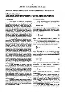
𝑥𝑖 ≤ 𝛼𝑖 𝑥𝑖𝑈 + (1 − 𝛼𝑖 ) 𝑥𝑖𝑏 , 𝛼𝑖 = 0 or 𝛼𝑖 = 1, 𝑦𝑒 = 𝑦𝑒,𝑑 ∈ {𝑦𝑒,1 , . . . , 𝑦𝑒,𝑝𝑒 } 𝑑 = 1, . . . , 𝑝𝑒 ; 𝑒 = 1, . . . , 𝑚, where 𝑊 is the total weight of the truss structure and 𝑓𝑖 (𝑋, 𝑌) denotes the weight of 𝑖th group. 𝑔𝑗 (𝑋, 𝑌) represents 𝑗th constraint in the model, which could be constraints of element stresses, node displacements, mode frequency, or buckling factor. 𝑘 denotes the total number of constraints, and V is the number of frequency or bulking constraints. If some bar members are removed, the corresponding constraints are eliminated, such as the stress constraints of the removed members. Thus, 𝛽𝑗 indicates whether the respective constraint is eliminated; if 𝛽𝑗 = 0, 𝑗th constraint is eliminated; otherwise if 𝛽𝑗 = 1, 𝑗th constraint is retained. To facilitate describing the optimization model, a truss structure is taken as an example, which is shown in Figure 1. 𝑦 coordinate of node 1 could be 100, 120, 140, and 160, while 𝑥 coordinate of node 2 could be 200, 240, and 280. It is required that the coordinate variation of node 1 and node 2 is independent and that node 1 should be symmetric with node 3 along the dotted line, which means that there are two independent shape variables. In addition, the cross-sectional dimension of each bar element is required to be optimized independently and each bar element is allowed to be deleted or retained, which means that there are 7 size variables and 7 topology variables.

3. Optimization Method 3.1. The First-Level Approximate Problem. To solve problem (1) which is always implicit, a first-level problem is constructed to transform 𝑓𝑖 (𝑋) and 𝑔𝑗 (𝑋) into a sequence of

Mathematical Problems in Engineering

3 1

A1

5

A5

A6

A2 2

60

120

A7

Y

A3

A4

120

120

X

4

3

Coordinates 1 (120, 120, 0), 2 (240, 60, 0), 3 (120, 0, 0), 4 (0, 0, 0), 5 (0, 120, 0)

Figure 1: Seven-bar truss and node coordinates.

nonlinear explicit approximate functions. In 𝑝th stage, the approximate explicit problem can be stated as Find

𝑋 = {𝑥1 , 𝑥2 , . . . , 𝑥𝑛 } , 𝑇

𝑌 = {𝑦1 , 𝑦2 , . . . , 𝑦𝑚 } , 𝑇

(𝑝)

(𝑋)

𝑖=1

s.t.

(𝑝) 𝛽𝑗 𝑔𝑗

ℎ𝑡 (𝑋) =

(𝑋) ≤ 0 𝑗 = 1, . . . , 𝐽1 ,

(𝑝)

𝑔𝑗 (𝑋) ≤ 0 𝑗 = 𝐽1 + 1, . . . , 𝐽, 𝐿 𝛼𝑖 𝑥𝑖(𝑝)

+ (1 −

𝛼𝑖 ) 𝑥𝑖𝑏

≤ 𝑥𝑖

(2)

𝑡=𝑝−(𝐻−1)

𝑛

{𝑔𝑗 (𝑋𝑡 ) + ∑𝑔̃𝑗,𝑖,𝑡 (𝑋)} ℎ𝑡 (𝑋) , 𝑖=1

ℎ𝑡 (𝑋) 𝐻 ∑𝑙=1 ℎ𝑙 (𝑋) 𝐻

𝑡 = 1, . . . , 𝐻,

(5)

(6)

(7)

𝑇

ℎ𝑙 (𝑋) = ∏ (𝑋 − 𝑋𝑠 ) (𝑋 − 𝑋𝑠 ) ,

(8)

𝑠=1,𝑠=𝑙̸

𝑖 = 1, . . . , 𝑛,

𝐻

2

min √ { ∑ 𝑔𝑗 (𝑋𝑧 ) − 𝑔𝑗 (𝑋𝑡 ) − 𝑔̃𝑗,𝑖,𝑡 (𝑋𝑡 )}

𝑈 𝑥𝑖 ≤ 𝛼𝑖 𝑥𝑖(𝑝) + (1 − 𝛼𝑖 ) 𝑥𝑖𝑏 ,

𝑧=1

𝛼𝑖 = 0 or 𝛼𝑖 = 1,

s.t.

𝑦𝑒 = 𝑦𝑒,𝑑 ∈ {𝑦𝑒,1 , . . . , 𝑦𝑒,𝑝𝑒 }

(9)

− 5 ≤ 𝑟𝑜,𝑡 ≤ 5, − 5 ≤ 𝑟𝑚,𝑡 ≤ 5, 𝑡 = 1, . . . , 𝐻,

𝑑 = 1, . . . , 𝑝𝑒 ; 𝑒 = 1, . . . , 𝑚, 𝑈 𝑈 𝑥𝑖(𝑝) = min {𝑥𝑖𝑈, 𝑥̃𝑖(𝑝) },

(3)

𝐿 𝐿 𝑥𝑖(𝑝) = max {𝑥𝑖𝐿 , 𝑥̃𝑖(𝑝) },

(4)

𝑈 𝐿 where 𝑥𝑖(𝑝) and 𝑥𝑖(𝑝) are upper and lower bounds of size var𝑈 𝐿 and 𝑥̃𝑖(𝑝) are the moving limits of 𝑥𝑖 iable 𝑥𝑖 at 𝑝th stage; 𝑥̃𝑖(𝑝) (𝑝)

∑

1 𝜕𝑔𝑗 (𝑋𝑡 ) 1−𝑟𝑜,𝑡 𝑟𝑜,𝑡 𝑟 { 𝑥𝑖𝑡 (𝑥𝑖 − 𝑥𝑖𝑡𝑜,𝑡 ) , if 𝛼𝑖 = 1 { { { 𝑟𝑜,𝑡 𝜕𝑥𝑖 𝑔̃𝑗,𝑖,𝑡 (𝑋) = { { 1 𝜕𝑔𝑗 (𝑋𝑡 ) { { (1 − 𝑒−𝑟𝑚,𝑡 (𝑥𝑖 −𝑥𝑖𝑡 ) ) , if 𝛼𝑖 = 0, { 𝑟𝑚,𝑡 𝜕𝑥𝑖

𝛼 = {𝛼1 , 𝛼2 , . . . , 𝛼𝑛 } , 𝑛

𝑝

(𝑝)

𝑔𝑗 (𝑋) =

𝑇

min 𝑊 = ∑𝛼𝑖 𝑓𝑖

used to construct a branched multipoint approximate (BMP) function ((5)–(8)) [5, 12]:

at 𝑝th stage; 𝑔𝑗 (𝑋) are 𝑗th approximate constraint function at 𝑝th stage, which is constructed as follows. First, structural and sensitivity analysis are implemented at the point 𝑋(𝑝) = {𝑥1(𝑝) , 𝑥2(𝑝) , . . . , 𝑥𝑛(𝑝) }𝑇 to obtain the constraint response. Second, the results of structural and sensitivity analysis are

where 𝑋𝑡 is 𝑡th known point, 𝐻 is the number of points to be counted, and 𝐻 = min{𝑝, 𝐻max }. When the number of known points is larger than 𝐻max (always set as 5), only the last 𝐻max points are counted; ℎ𝑡 (𝑋) is a weighting function, which is defined in (7)-(8); 𝑟𝑜,𝑡 and 𝑟𝑚,𝑡 are the adaptive parameter (𝑝) controlling the nonlinearity of 𝑔𝑗 (𝑋), which are determined by solving the least squares parameter estimation in (9). When 𝑡 = 1, 𝑟𝑜,𝑡 = −1 and 𝑟𝑚,𝑡 = 3.5. For more details of BMP function, please see the work by Dong and Huang (2004) [12]. Though problem (2) is explicit, it involves topology and shape variables which cannot be directly solved by mathematical programming method. Thus a GA is implemented for explicit mixed variables problem (2).

4

Mathematical Problems in Engineering

3.2. GA to Deal with Mixed Variables Problem. GA is used to generate and operate on sequences of mixed variables vector 𝑆 = {𝑦1 , 𝑦2 , . . . , 𝑦𝑚 , 𝛼1 , 𝛼2 , . . . , 𝛼𝑛 }𝑇 representing the truss shape and topology, in which 𝛼𝑖 (𝑖 = 1, . . . , 𝑛) is 0/1 variables and 𝑦𝑑 (𝑑 = 1, . . . , 𝑚) is integer-valued variable. ∗ obtained in the last Based on the optimum vector 𝑆𝑝−1 iteration, the GA generates an initial population randomly, in which the vector 𝑆𝑙,𝑘,𝑝 (𝑘 = 1) represents 𝑙th individual in 𝑘th generation at 𝑝th iteration of the first-level approximate problem. Then, for every individual in the current generation, ∗ is obtained by solving a the optimal size variables vector 𝑋𝑙,𝑘,𝑝 second-level approximation problem, which will be described later in Section 3.3. To reduce the structural analyses, the ∗ ) is calculated accurately with objective value 𝑊(𝑝) (𝑋𝑙,𝑘,𝑝

a, b, c, d, e, f1 , . . . , fd

Node ID Number of node The coordinate value of point 1 coordinate values

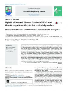
Figure 2: The definition of shape variables.

s.t.

(𝑝)

∗ analytic expressions, and the constraint value 𝑔𝑗 (𝑋𝑙,𝑘,𝑝 ) is calculated with approximate functions ((5)–(9)). Then, (𝑝) ∗ ∗ 𝑊(𝑝) (𝑋𝑙,𝑘,𝑝 ) and 𝑔𝑗 (𝑋𝑙,𝑘,𝑝 ) are used to calculate the fitness of individual 𝑋𝑙,𝑘,𝑝 with penalty function method (10). For more details of penalty functions, please see work by Li et al. (2014) [5]. Consider 󵄨󵄨 󵄨󵄨 𝐽1 󵄨󵄨𝑔𝑗 󵄨󵄨 ∗ ∗ 󸀠 ), penal (𝑋𝑙,𝑘,𝑝 ) = 𝑊 ∑ 𝐽󵄨 󵄨 2 V𝑗 (𝑋𝑙,𝑘,𝑝 1 𝑔 ∑ 𝑗=1 𝑗=1 𝑗 ∗ ) fitness (𝑋𝑙,𝑘,𝑝

=

𝑝 {𝑓max

⋅ (1 +

(10) (𝑝)

− (𝑊

∗ (𝑋𝑙,𝑘,𝑝 )

+

∗ penal (𝑋𝑙,𝑘,𝑝 ))}

𝑀crit ). 𝐽1

After the fitness value of all the members in the initial generation is calculated, the genetic selection, crossover, and mutation operators work on the vector 𝑆𝑙,𝑘,𝑝 in sequence ∗ ) to generate based on the individual fitness value fitness(𝑋𝑙,𝑘,𝑝 the next generation (𝑘 = 𝑘 + 1). The different genetic operations on 0/1 variables vectors 𝛼 = {𝛼1 , 𝛼2 , . . . , 𝛼𝑛 }𝑇 and integer-valued variables vectors 𝑌 = {𝑦1 , 𝑦2 , . . . , 𝑦𝑚 }𝑇 will be described in Section 4. When the maximum generation (max 𝐺) is reached, the optimum vectors 𝑆𝑝∗ and 𝑋𝑝∗ are obtained for the next iteration (𝑝 = 𝑝 + 1) of the first-level approximate problem. 3.3. The Second-Level Approximate Problem. After constructing first-level approximate problem (2) and implementing GA to generate sequences of vector 𝑆𝑙,𝑘,𝑝 , original problem (1) is transformed to an explicit problem with continuous size variables only. To improve the computational efficiency, a second-level approximate problem is constructed using linear Taylor expansions of reciprocal design variables [5, 12]. In 𝑚th step, the second-level approximate problem is stated in ̃ min 𝑊(𝑚) (𝑋) 𝐷

̃ (𝑋 ̃(𝑚) ) + ∑ =𝑊

𝑑=1

̃ (𝑋 ̃(𝑚) ) 𝜕𝑊 𝜕𝑥̃𝑑

(𝑥̃𝑑 − 𝑥̃𝑑(𝑚) )

The coordinate value DOF of point d Starting point ID

Variable ID

̃ 𝑔𝑗(𝑚) (𝑋) ̃(𝑚) ) = 𝑔̃𝑗 (𝑋 𝐷

2 − ∑ 𝑥̃𝑑(𝑚) 𝑑=1

̃(𝑚) ) 𝜕𝑔̃𝑗 (𝑋 𝜕𝑥̃𝑑

(

1 1 − )≤0 𝑥̃𝑑 𝑥̃𝑑(𝑚) 𝑗 = 1, . . . , 𝐽2 ,

𝑥𝐿𝑑(𝑚) ≤ 𝑥̃𝑑 ≤ 𝑥𝑈 𝑑(𝑚)

𝑑 = 1, . . . , 𝐷, (11)

̃ is the approximate objective value and where 𝑊(𝑚) (𝑋) (𝑚) ̃ 𝑔 (𝑋) is the approximate value of 𝑗th constraint in 𝑚th step; 𝑗

𝑈 𝐿 ̃𝑑 and 𝑥𝑈 and 𝑥𝐿 are 𝑥̃𝑑(𝑚) and 𝑥̃𝑑(𝑚) are move limits of 𝑋 𝑑(𝑚) 𝑑(𝑚) upper and lower bounds of 𝑥𝑑 in 𝑚th step. After constructing the second-level approximate problem, a dual method and a ∗ [5, 12]. BFGS are used to seek the optimal size variable 𝑋𝑙,𝑘,𝑝

4. Improvements in GATA for Adding Shape Variables To facilitate describing the improvements for adding shape variables in GATA, the truss structure in Figure 1 is also taken as an example. 4.1. Definition of Shape Variables and Variable Link. In problem (1), 𝑌 = {𝑦1 , 𝑦2 , . . . , 𝑦𝑚 }𝑇 is the shape variable vector; 𝑦𝑒 = 1 ∼ 𝑝𝑒 (𝑒 = 1, 2, . . . , 𝑚) denotes the identifier number of the possible coordinates. Each shape variable is defined with an array. As shown in Figure 2, 𝑎 represents the identifier number of shape variables; 𝑏 is the identifier number of the nodes to be moved; 𝑐 means the direction of coordinate, which could be 1 or 2 or 3, corresponding to 𝑥- or 𝑦- or 𝑧-axis coordinate, respectively; 𝑑 is the number of possible discrete coordinate values of node 𝑑; 𝑒 denotes the identifier number of node coordinates of the initial truss structure; {𝑓1 , 𝑓2 , . . . , 𝑓𝑑 } denotes the discrete coordinate set of node 𝑏, or variable 𝑎, and 𝑓1 ≤ 𝑓2 ≤ ⋅ ⋅ ⋅ ≤ 𝑓𝑑 (or 𝑓1 ≥ 𝑓2 ≥ ⋅ ⋅ ⋅ ≥ 𝑓𝑑 ). The shape variables can be linked with each other; that is, some node coordinates could vary with a given relation, such as symmetric variation. The definition of shape variable link relation is explained in Figure 3. 𝑎 represents the identifier

Mathematical Problems in Engineering Variables ID Orientation

5 1

3

1

1

1

1

1

0

1

a, b, c, Δd

Node ID

Moving scale coefficient

Figure 3: The link method of shape variables.

number of shape variables; 𝑏 is the identifier number of the nodes that is expected to link; 𝑐 denotes the direction of coordinate which is expected to link, 𝑐 = 1 or 2 or 3, corresponding to 𝑥- or 𝑦- or 𝑧-axis coordinate, respectively; Δ𝑑 is defined as a moving scaling factor, which means that the linked coordinate value is Δ𝑑 ⋅ 𝑥 when the coordinate value of shape variable 𝑎 is 𝑥; Δ𝑑 = −1 for symmetric nodes. According to the shape variable definition rules described above, the shape variables of node 1 and node 2 could be defined as follows: 1, 1, 2, 4, 2, 100, 120, 140, 160, 2, 2, 1, 3, 2, 200, 240, 280. The node 3 is symmetric with node 1 along the dotted line in Figure 1; thus, a sentence should be defined to describe the shape variable link relationship; that is, 1, 3, 2, −1. The definitions of shape variables and variable link are further explained in Figures 2 and 3, respectively. 4.2. GA Execution Process 4.2.1. Hybrid Coding Strategy of Shape and Topology Variables. In GATA, discrete variables are optimized through GA. After introducing the discrete shape variables, the string of genes should include the information of both topology variables and shape variables. Decimal coding is adopted for nodal positions, while the topology variables keep using binary format. The gene of each individual could be written as 𝑆 = 𝑦1 𝑦2 ⋅ ⋅ ⋅ 𝑦𝑚 𝛼1 𝛼2 ⋅ ⋅ ⋅ 𝛼𝑛 where 𝑦1 𝑦2 ⋅ ⋅ ⋅ 𝑦𝑚 and 𝛼1 𝛼2 ⋅ ⋅ ⋅ 𝛼𝑛 represent the code of shape variables and topology variables, respectively. For instance, there are 2 shape variables and 7 topology variables in the truss of Figure 1; the gene of an individual is 1-3-1-1-1-1-1-0-1, which means the first shape variable taking the 1st coordinate in {100, 120, 140, 160} and the second shape variable taking the 3rd coordinate in {200, 240, 280}. The corresponding truss configuration is shown in Figure 4. 4.2.2. Generation of the Initial Population. The generation mechanism of the initial population is updated for involving shape variables. At the first/initial calling of GA, the initial population of the designs is generated randomly. Once the optimal members of the population have been obtained, the initial population of the next generation is generated

Shape variables

Topology variables

Figure 4: Example of individual gene code.

according to the elite of former generations of the GA. That is to say, from the second calling of the GA, the initial population consists of three parts: (1) there are the optimal individuals of the former generations; (2) members which are generated according to the optimal individuals of the last generation; that is, 𝑦𝑖 (𝑖 = 1, . . . , 𝑚) sequentially mutate under control with a low probability (Section 4.2.4), while 𝛼𝑖 will approach 0 with a greater probability if the corresponding optimal size variable 𝑥𝑖 is small; (3) the mutation of 𝑦𝑖 is the same as that in (2), while 𝛼𝑖 mutate randomly with a given low probability. The mutation control technique of shape variables will be explained in Section 4.2.4. According to our calculation experience, the population size and maximum evolutional generation should exceed twice the total design variables. If it is more than 100, then it will take 100. 4.2.3. Roulette-Wheel Selection. Roulette-wheel selection is used to select a father design and a mother design from the parent generation, which is easy to be executed. Suggesting that the population size is 𝑀, the fitness value of 𝑖th individual in 𝑘th generation is 𝐹𝑖 ; then the probability of individual 𝑖 to be selected in the next generation is 𝑃𝑖𝑠 =

𝐹𝑖 𝑀 ∑𝑖=1

𝐹𝑖

.

(12)

It can be seen from (12) that the individual of higher fitness value has greater probability to be selected. The fitness value of each individual is obtained using (10), as described in Section 3.2. 4.2.4. Uniform Crossover. Uniform crossover is popularly applied in the GA since it could produce better individuals and has lower probability to break good individuals. Since decimal coding is adopted for nodal coordinates, while the topology variables keep using binary format, crossover operator could not be carried on between these two kinds of code. Uniform crossover which operates gene by gene is implemented to the two areas independently. Before crossover, two individuals are selected randomly as mother and father chromosomes. Then, for each gene, a random value 𝑟 within 0∼1 is generated. Let 𝑥1 = value of gene from the mother and let 𝑥2 = value of gene from the father. Let 𝑦1 = value of gene from the first child and let 𝑦2 = value of gene

6

Mathematical Problems in Engineering

from the second child. For 0/1 topology genes and integervalued shape genes, 𝑦1 = 𝑥1 , 𝑦2 = 𝑥2 , if 𝑟 > 𝑃𝑐 𝑦1 = 𝑥2 ,

(13)

𝑦2 = 𝑥1 , if 𝑟 ≤ 𝑃𝑐 , where 𝑃𝑐 is the crossover probability. Repeat this process until a new population is generated with 𝑁 individuals. 4.2.5. Controlled Uniform Mutation of Shape Variables. Uniform mutation and controlled uniform mutation are implemented for 0/1 topology genes and integer-valued genes, respectively. For each gene, a random number 𝑟 between zero and one is generated. If 𝑟 ≤ 𝑃mutate (mutating probability), the gene is mutated. For 0/1 valued topology genes, the gene is mutated to its allelomorph (0 → 1, 1 → 0). For an integer-valued coordinate gene, a controlled mutation technique is implemented to limit the mutation range, which could decrease the numerical instability induced by the large change of coordinates and improve the accuracy of the firstlevel approximation functions. Two parameters are included in the control mutation technique, which are mutation probability 𝑃𝑚 and move limit 𝑃move . Mutation operation is implemented to each point of shape gene sequentially with 𝑃𝑚 . First, if a particular point needs to mutate, let us assume that the number of coordinate positions with respect to this shape variable is 𝑑 and the present identifier number is 𝑒, and then the upper limit UPmute and lower limit DOmute of allowable mutation range are obtained as {min ([𝑑 ⋅ 𝑃move ] + 𝑒, 𝑑) UPmute = { min (1 + 𝑒, 𝑑) {

𝑑 ⋅ 𝑃move ≥ 1

{max ([𝑒 − 𝑑 ⋅ 𝑃move ] , 1) ={ max (𝑒 − 1, 1) {

𝑑 ⋅ 𝑃move ≥ 1

DOmute

the last iteration. Therefore, it is necessary to update the firstlevel approximation problem, so as to make it correspond to the present shape. The update strategy of the first-level approximation problem is then modified as follows. If the shape code of the optimal individual is inconsistent with that of the last iteration, a new first-level approximation problem will be built, and the number of known points 𝐻 will be set as 1; else the first-level approximation problem is consistent with the last iteration and increases the number of known points 𝐻. The update strategy of the first-level approximate problem in the whole optimization process is emphasized in the algorithm flowchart (Figure 5). 4.4. Algorithm Flowchart. The flowchart of the IGATA (Improved Genetic Algorithm with Two-Level Approximation) for truss size/shape/topology optimization is shown in Figure 5. After getting the optimal 𝑋𝑝∗ from the GA, a convergence criterion in (15) is used to determine whether the first-level approximate problem is terminated. Here, 𝜀1 is size variables convergence control parameter, 𝜀3 is weight convergence control parameter, 𝜀2 is the constraints control parameter, and 𝑝max is the maximum iterative number for first-level approximate problem. The computational cost of IGATA is low because the first-level approximate techniques reduce the number of structural analyses significantly and the second-level approximate techniques reduce the number of the design variables significantly [5, 12]: 󵄨󵄨 𝑥𝑖𝑝 − 𝑥𝑖(𝑝−1) 󵄨󵄨 󵄨󵄨 󵄨󵄨 󵄨󵄨 ≤ 𝜀1 󵄨󵄨 󵄨󵄨 󵄨󵄨 𝑥𝑖1

(𝑖 = 1, 2, . . . , 𝑛) ,

𝑔max (𝑋𝑝 ) = max (𝑔1 (𝑋𝑝 ) , . . . , 𝑔𝑚 (𝑋𝑝 )) ≤ 𝜀2 or 𝑝 = 𝑝max ,

(15)

󵄨󵄨 󵄨 󵄨󵄨 𝑊 (𝑋𝑝 ) − 𝑊 (𝑋𝑝−1 ) 󵄨󵄨󵄨 󵄨󵄨 󵄨󵄨 ≤ 𝜀 . 󵄨󵄨 󵄨󵄨 3 󵄨󵄨 󵄨󵄨 𝑊 (𝑋𝑝 ) 󵄨 󵄨

5. Numerical Examples

𝑑 ⋅ 𝑃move ≤ 1, (14) 𝑑 ⋅ 𝑃move < 1.

Note that [𝑥] denotes the maximum integer not larger than 𝑥. Then, an integer between UPmute and DOmute will be generated as the mutation result. Normally, 𝑃𝑚 = 0.001∼0.5 and 𝑃move = 0.3∼0.5. 4.3. Update Strategy of the First-Level Approximation Problem. In 𝑝th iteration process of GATA for truss shape and topology optimization, the results of the structural and sensitivity analysis at 𝑋𝑝 are used to construct the first-level approximation problem using the multipoint approximation function. After introducing the shape variables, the truss shape 𝑌 = {𝑦1 , 𝑦2 , . . . , 𝑦𝑚 }𝑇 |𝑝 might be different from that in

5.1. Ten-Bar Truss. The ten-bar truss has been studied by Rajan [6], as shown in Figure 6. The unit of length is inch. Node 6 is the original point. The length of bars 1, 2, 3, 4, 5, and 6 is 360 in. Nodes 4 and 6 are separately applied to a force of 100000 lb. Young’s modulus is 𝐸 = 107 Psi and material density is 0.1 lb/in.3 . The section area of each bar is taken as independent variable, which is originally 10 in.2 and is permitted to vary between 1 in.2 and 34 in.2 . 𝑦 coordinates of nodes 1, 3, and 5 are taken as independent shape variables. The moveable range of 𝑦 coordinate is 180 in. to 1000 in. Discrete coordinates are preset for the shape variables, as shown in Table 1. The shape variables and link relation are defined as definition. Therefore, there are 10 size variables, 10 topology variables, and 3 shape variables in all. The stress of each bar should not exceed ±25,000 Psi. The parameters of GA are set as follows: population size 30, evolution generations 35, crossover probability 0.8, and mutation probability 0.05. The optimized solution of

Mathematical Problems in Engineering

7

Generate the initial population (k = 1)

Initial design X1

Execute structure analysis and sensitivity analysis at point Xp (p = 1) Executing updating strategy of the firstlevel approximation problem

Execute selecting, crossing, and mutating action to generate the next generation (k = k + 1)

Establish the first-level approximation problem

No

Yes

Execute GA

Yes

Establish the second-level approximation problem for every individual

Calculate individual adapting fitness

Use dual method and BFGS method to optimize size variables

The second-level converged?

k < maxG?

Are YP and YP−1 the same?

No No

Execute elite selection strategy (p = p + 1)

The first-level terminated? Yes

∗ Get the optimal Xl,k,p

Get the optimal Sp∗

Get the optimal X∗

Sizing optimization

Truss shape and topology optimization

Figure 5: The flowchart of the present approach.

1

5

2

3

9

7 5

8

6

1

6

10

4

3

4

100000 lb

2

100000 lb

Figure 6: Ten-bar truss structure.

the shape, topology, cross-sectional areas, structural weight, and constraint obtained by the present approach is listed in Table 2, for comparison with [6]. It is seen from Table 2 that the critical constraint is very close to the boundary and the optimal weight of this paper is 3173 lb, which is lower than the result of [6] by 81 lb. The optimized shape and topology configuration are contrasted in Figure 7. The iteration history is shown in Figure 8. It is seen that the optimized solution is obtained after only 4 iterations. This example demonstrated the validity and efficiency of the proposed method. 5.2. Twelve-Bar Truss. A twelve-bar truss has been studied by Zhang et al. [13], as shown in Figure 9. The unit of length is mm. The structural symmetry should be kept in the design process. Young’s modulus is 𝐸 = 1000 Pa and material

density is 1 kg/mm3 . The section area of each bar is taken as independent variable, which is originally 10 mm2 , and is permitted to vary between 1 mm2 and 100 mm2 . 𝑥 and 𝑦 coordinates of nodes 2 and 5 are taken as independent shape variables. The moveable range of 𝑥 coordinate is 0 mm to 50 mm, and the moveable range of 𝑦 coordinate is 0 to ∞. Discrete coordinates are preset for the shape variables, as shown in Table 3. The shape variables and link relation are defined as definition. Therefore, there are 12 size variables, 12 topology variables, and 4 shape variables in all. The stress of each bar should not exceed ±450 Pa. The parameters of GA are set as follows: population size 50, evolution generations 50, crossover probability 0.9, and mutation probability 0.05. The optimized solution of the shape, topology, cross-sectional areas, structural weight,

8

Mathematical Problems in Engineering

+

+

(a) Optimal shape and topology in this paper

(b) Optimal shape and topology in [6]

Figure 7: The optimized shape and topology of ten-bar truss structure.

Table 1: Shape variables and coordinates identifier number.

1 2 3

𝑦1 𝑦3 𝑦5

Position number and corresponding coordinates 1

2

3

360 610 687 300 330 360 180 187 190

4

5

6

7

8

760 450 200

787 540 210

810 554 230

860 560 260

1000 360

Note: S.V. are shape variables.

4400 4200 4196.5 Weight (kg)

S.V. ID Coord.

Table 2: Comparison of optimized design of ten-bar planar truss. Variable Initial design 𝑦1 360 360 𝑦3 360 𝑦5 10 𝐴1 10 𝐴2 10 𝐴3 10 𝐴4 10 𝐴5 10 𝐴6 10 𝐴7 10 𝐴8 10 𝐴9 10 𝐴 10 Struc. analyses Weight (lb) Critical constraint

Present paper 180 330 687 21.6 1.0 12.6 12.6 4.4 17.1 0 2.6 0 1.0 20 3173.0 2.1 × 10−4

Reference [6] 186.5 554.5 786.9 9.9 9.4 11.5 1.5 0 12.0 11.5 3.6 0 10.4 — 3254.0 —

and constraint obtained by the present approach is listed in Table 4, for comparison with [13]. The optimized shape and topology configuration are contrasted in Figure 10. The iteration history is shown in Figure 11. It is seen that the final structural weight is 1023 kg, which is lower than the result in [13] by 109 kg, and the critical constraint is very close to the boundary. The optimized solution is obtained after only 4 iterations. This example demonstrated the validity and efficiency of the proposed method.

4592.3

4600

4000 3800 3600

3512.5

3400 3204.5

3200 3000

1

0

2

3172.9

3

4

Iteration number

Figure 8: Iteration history of ten-bar truss.

Table 3: Shape variables and coordinates identifier number of 12-bar planar truss. S.V. ID Coord. 1 2 3 4

𝑥1 𝑥2 𝑦1 𝑦2

Position number and corresponding coordinates 1

2

3

4

5

5 30 2 2

10 35 5 5

15 40 10 10

20 45 15 15

25 20 20

6

7

25 25

30 30

6. Algorithm Performance Consider the example of ten-bar truss in Section 5, with population size and maximum generations (max 𝐺) set from 10 to 100, respectively, which is shown in Figure 12, while other parameters remain as given before. At each parameter set point, 100 independent runs of IGATA are executed. Since there are 100-parameter set points, IGATA is executed in a total of 10,000 times. For each parameter set point, the average weight is shown in Figure 13.

Mathematical Problems in Engineering

9 A(x1 , y1 )

E

C(x2 , y2 )

3

1

5

Y

11

Py = 2000 N

9 7

X

8

P

A7

G

Px = 5000 N

12 6 F

2 B(x1 , −y1 )

4

D(x2 , −y2 )

50

Figure 9: Twelve-bar truss structure.

Table 4: Comparison of optimized design of twelve-bar planar truss. Variable Initial design 𝑥1 15 30 𝑥2 15 𝑦1 15 𝑦2 10 𝐴1 10 𝐴2 10 𝐴3 10 𝐴4 10 𝐴5 10 𝐴6 10 𝐴7 10 𝐴8 10 𝐴9 10 𝐴 10 10 𝐴 11 10 𝐴 12 Struc. analyses Weight (kg) Critical constraint

Present paper 10 35 10 5 4.11 15.90 1.13 14.73 1.17 12.88 0 1.00 3.23 1.74 2.59 0 17 1023.3 2.1 × 10−4

Reference [13] 31.18 38.30 9.21 7.28 1.00 14.50 1.98 10.60 2.10 10.80 1.46 1.00 5.73 2.51 1.00 1.00 — 1132.6 —

It can be seen from Figure 13 that the minimum weight is 2800 lb, which is less than the weight of the initial structure by 32.6%. To describe the efficiency of the IGATA involving size/shape/topology variables, we counted the number of the results that are lower than 3254 lb, which is the optimal result in [6]. It can be seen that 8 results with lower weight are obtained within the 100-parameter set points. As compared with the IGATA only including size and topology variables [5], the algorithm performance in this paper is not so satisfactory. To test the reason for this situation, continuous shape variables instead of discrete variables were used in the hybrid coding strategy in GA. The results of repeated tests show that the algorithm performance does not improve obviously. Thus the main reason may not lie in

the continuity of shape variables but lie in the quality of the first-level approximation function induced by the shape variables. When executing GA in 𝑝th iteration process of IGATA for truss shape and topology optimization, the objective and constraint approximation functions of the optimal individual from the last iteration are used, which do not change along with the structure shape, although controlled mutation has been implemented. To improve the accuracy and efficiency of IGATA, we will use continuous shape variables and add sensitivity information of shape variables in the first-level approximation problem in the subsequent work.

7. Conclusion In this paper, aiming at simultaneous consideration of sizing, shape, and topology optimization of truss structures, a design method IGATA is presented, which is based on the truss sizing and topology optimization method GATA. The shape variables are involved by using GA and are considered as discrete to avoid the sensitivity calculation, through which the computational cost is decreased significantly. A comprehensive model is established for involving the three kinds of design of variables, in which the shape variables are corresponding to a set of discrete node coordinates. GA is used to solve the first-level approximate problem which involves sizing/shape/topology variables. When calculating the fitness value of each member in the current generation, a secondlevel approximation method is used to optimize the continuous size variables. The definition, link, and code of the shape variables are presented, and the crossover and mutation of the decimal/binary mix-coding population are realized. The update strategy of the first-level approximation problem is also improved for the cases when the truss shapes are different from the neighbor iterations, so as to ensure that the truss shape is corresponding with the approximation problem. The results of numerical example demonstrated the validity of the method. Moreover, truss optimization problem with sizing/shape/topology variables can be treated effectively with the proposed method.

10

Mathematical Problems in Engineering

+

+

(a) Optimal shape and topology in this paper

(b) Optimal shape and topology in [13]

Weight (kg)

Figure 10: The optimized shape and topology of twelve-bar truss structure.

Nomenclature

3000 2970.1 2800 2600 2400 2200 2000 1800 1600 1400 1200 1000 0 0.5

𝑋: 𝑥𝑖 :

1627.4 1188.2 1

1.5

2

2.5

1033.7 3 3.5

1023.3 4

Iteration number

Figure 11: Iteration history of twelve-bar truss.

Size variable vector Cross-sectional area of bar members in 𝑖th group 𝑌: Shape variable vector Identifier number within the possible 𝑦𝑒 : coordinates set [𝑦𝑒,1 , . . . , 𝑦𝑒,𝑝𝑒 ] 𝑎: Topology variable vector 𝑊: Total weight of the truss structure 𝑓𝑖 (𝑋, 𝑌): The weight of 𝑖th group 𝑔𝑗 (𝑋, 𝑌): 𝑗th constraint 𝑘: The total number of constraints V: The number of frequency constraints.

Conflict of Interests Parameter set point of popsize and maxG

110

The authors declare that there is no conflict of interests regarding the publication of this paper.

100 90

Acknowledgment

80 Popsize

70

This research work is supported by the National Natural Science Foundation of China (Grant no. 11102009), which the authors gratefully acknowledge.

60 50 40

References

30 20 10 0

20

0

40

60 maxG

80

100

Average weight

Figure 12: GA parameters set point.

5000 4000 3000 2000 100

80

60 max 40 G

20

0 0

80 60 40 ze psi 20 Po

Figure 13: Average weight at each set point.

100

[1] L. Wei, T. Tang, X. Xie, and W. Shen, “Truss optimization on shape and sizing with frequency constraints based on parallel genetic algorithm,” Structural and Multidisciplinary Optimization, vol. 43, no. 5, pp. 665–682, 2011. [2] D. Wang, W. H. Zhang, and J. S. Jiang, “Truss optimization on shape and sizing with frequency constraints,” AIAA Journal, vol. 42, no. 3, pp. 622–630, 2004. [3] O. Sergeyev and Z. Mr´oz, “Sensitivity analysis and optimal design of 3D frame structures for stress and frequency constraints,” Computers and Structures, vol. 75, no. 2, pp. 167–185, 2000. [4] R. Su, X. Wang, L. Gui, and Z. Fan, “Multi-objective topology and sizing optimization of truss structures based on adaptive multi-island search strategy,” Structural and Multidisciplinary Optimization, vol. 43, no. 2, pp. 275–286, 2011. [5] D. Li, S. Chen, and H. Huang, “Improved genetic algorithm with two-level approximation for truss topology optimization,” Structural and Multidisciplinary Optimization, vol. 49, no. 5, pp. 795–814, 2014.

Mathematical Problems in Engineering [6] S. D. Rajan, “Sizing, shape, and topology design optimization of trusses using genetic algorithm,” Journal of Structural Engineering, vol. 121, no. 10, pp. 1480–1487, 1995. [7] R. J. Balling, R. R. Briggs, and K. Gillman, “Multiple optimum size/shape/topology designs for skeletal structures using a genetic algorithm,” Journal of Structural Engineering, vol. 132, no. 7, Article ID 015607QST, pp. 1158–1165, 2006. [8] P. Hajela and E. Lee, “Genetic algorithms in truss topological optimization,” International Journal of Solids and Structures, vol. 32, no. 22, pp. 3341–3357, 1995. [9] H. Kawamura, H. Ohmori, and N. Kito, “Truss topology optimization by a modified genetic algorithm,” Structural and Multidisciplinary Optimization, vol. 23, no. 6, pp. 467–472, 2002. [10] W. Tang, L. Tong, and Y. Gu, “Improved genetic algorithm for design optimization of truss structures with sizing, shape and topology variables,” International Journal for Numerical Methods in Engineering, vol. 62, no. 13, pp. 1737–1762, 2005. [11] K. Sawada, A. Matsuo, and H. Shimizu, “Randomized line search techniques in combined GA for discrete sizing optimization of truss structures,” Structural and Multidisciplinary Optimization, vol. 44, no. 3, pp. 337–350, 2011. [12] Y. Dong and H. Huang, “Truss topology optimization by using multi-point approximation and GA,” Chinese Journal of Computational Mechanics, vol. 21, no. 6, pp. 746–751, 2004. [13] Z. Zhang, W. Yao, and L. Zhou, “Study on size and shape collaborative optimization mehtod of truss strucure,” Advances in Aeronautical Science and Engineering, vol. 3, no. 2, pp. 138–143, 2012.

11

Advances in

Operations Research Hindawi Publishing Corporation http://www.hindawi.com

Volume 2014

Advances in

Decision Sciences Hindawi Publishing Corporation http://www.hindawi.com

Volume 2014

Journal of

Applied Mathematics

Algebra

Hindawi Publishing Corporation http://www.hindawi.com

Hindawi Publishing Corporation http://www.hindawi.com

Volume 2014

Journal of

Probability and Statistics Volume 2014

The Scientific World Journal Hindawi Publishing Corporation http://www.hindawi.com

Hindawi Publishing Corporation http://www.hindawi.com

Volume 2014

International Journal of

Differential Equations Hindawi Publishing Corporation http://www.hindawi.com

Volume 2014

Volume 2014

Submit your manuscripts at http://www.hindawi.com International Journal of

Advances in

Combinatorics Hindawi Publishing Corporation http://www.hindawi.com

Mathematical Physics Hindawi Publishing Corporation http://www.hindawi.com

Volume 2014

Journal of

Complex Analysis Hindawi Publishing Corporation http://www.hindawi.com

Volume 2014

International Journal of Mathematics and Mathematical Sciences

Mathematical Problems in Engineering

Journal of

Mathematics Hindawi Publishing Corporation http://www.hindawi.com

Volume 2014

Hindawi Publishing Corporation http://www.hindawi.com

Volume 2014

Volume 2014

Hindawi Publishing Corporation http://www.hindawi.com

Volume 2014

Discrete Mathematics

Journal of

Volume 2014

Hindawi Publishing Corporation http://www.hindawi.com

Discrete Dynamics in Nature and Society

Journal of

Function Spaces Hindawi Publishing Corporation http://www.hindawi.com

Abstract and Applied Analysis

Volume 2014

Hindawi Publishing Corporation http://www.hindawi.com

Volume 2014

Hindawi Publishing Corporation http://www.hindawi.com

Volume 2014

International Journal of

Journal of

Stochastic Analysis

Optimization

Hindawi Publishing Corporation http://www.hindawi.com

Hindawi Publishing Corporation http://www.hindawi.com

Volume 2014

Volume 2014