Research Article Improved Genetic Algorithm with

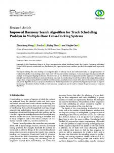
Hindawi Publishing Corporation Mathematical Problems in Engineering Volume 2015, Article ID 719409, 14 pages http://dx.doi.org/10.1155/2015/719409

Research Article Improved Genetic Algorithm with Gene Recombination for Bus Crew-Scheduling Problem Cuiying Song,1 Wei Guan,2 Jihui Ma,1 and Tao Liu3 1

MOE Key Laboratory for Urban Transportation Complex Systems Theory and Technology, School of Traffic and Transportation, Beijing Jiaotong University, 3 Shang Yuan Cun, Haidian District, Beijing 100044, China 2 Institute of Systems Engineering and Control, School of Traffic and Transportation, Beijing Jiaotong University, 3 Shang Yuan Cun, Haidian District, Beijing 100044, China 3 Department of Civil and Environmental Engineering, Transportation Research Centre, The University of Auckland, 20 Symonds Street, Auckland 1142, New Zealand Correspondence should be addressed to Wei Guan; [email protected] and Jihui Ma; [email protected] Received 8 December 2014; Accepted 9 April 2015 Academic Editor: Michael Small Copyright © 2015 Cuiying Song et al. This is an open access article distributed under the Creative Commons Attribution License, which permits unrestricted use, distribution, and reproduction in any medium, provided the original work is properly cited. This paper presents an improved genetic algorithm (GA) with gene recombination for bus crew-scheduling problem in bus company. Unlike existing methods that rely on designing a fixed potential shift set by software, our new method does not need such a potential shift set information. In our method, satisfied shifts are generated through gene recombination in genetic algorithm. We conduct extensive studies based on real-life instances from Beijing Bus Group. Compared with results generated by the current manual method, ant colony algorithm, and CPLEX, computational results show that our algorithms demonstrated very good computational performances. In our tests, the number of the maximum reducing shifts can be beyond 30, especially when trip number is very large. The high relative percentage deviation demonstrated the effectiveness of the algorithm proposed.

1. Introduction It has been known for more than 50 years [1] that the crew-scheduling problem for bus drivers (CSP-BD) is one of the most important operational-planning problems in a bus company, because, from the transit agencies’ perspective, the largest cost of providing service is generated by drivers’ wages and fringe benefits [2]. The CSP-BD is aimed at assigning vehicle trips to crews in such a way that each trip is covered by a shift, while guaranteeing that all other duty functions are feasible and the total cost of all duties is minimized [2–6]. CSP-BD has attracted the interest of many researchers since the 1960s, and research in this area has become very active since the 1990s. Most of the methods in the existing studies are based on mathematical programming or on hybrid approaches, which are combination of heuristics and Integer Linear Programming (ILP) [7–10]; the success and limitations of these methods have been discussed in Kwan et al. [11, 12] and Li and Kwan [13]. In the mathematical programmingbased approach, CSP-BD is formulated as covering/partition

problems that aimed at generating a subset of shifts to cover all pieces of trips, with the objective of minimizing total costs or total number of shifts [13]. In recent years, metaheuristics have been widely used for searching practical near-optimal solutions to NP-hard problems. Metaheuristics offer three main advantages: (a) they are usually very efficient in searching through very large solution space; (b) they can result in a feasible solution; (c) each class of metaheuristics has its own methodical and strategic structure. Until now, much effort has been made in exploring metaheuristics, such as tabu searches (TS) [9, 14, 15], ant system [16–18], and simulated annealing [19]. Genetic algorithms (GAs), one of the most important metaheuristics, form another major class for crew scheduling. In general, structure of GA for CSP-BD could be divided into two classes: one is the shift-based chromosome structure and the other is called the piece-based chromosome structure. In the shift-based structure, the chromosome length is not fixed. By changing the gene in chromosomes repeatedly through genetic operators, a feasible solution can be obtained [20, 21].

2 In the piece-based chromosome structure [22], a gene usually represents each piece. If a gene is chosen during the genetic operation, the corresponding shift covering the chosen gene will also be selected. Therefore, the simple crossover operation may be infeasible based on the units of shifts, let alone mutation. Furthermore, once a shift unit existed in a chromosome, no new shift units were produced except for exchanging the parent chromosomes. Thus, the efficiency of algorithm largely depends on initial parent chromosomes. Most of researches mentioned above were based on a pregenerated set of potential fixed shifts. Through adding or removing shift units during genetic operations, an optimum solution with the least shifts is obtained. Different from the above generated method, this work introduces a new method without using the potential shift set; instead, satisfied shifts generated from process of gene recombination in genetic algorithm are employed. A different piece-based structure is taken into account and the optimal solution is generated by repeated recombination process. The rest of paper is organized as follows. Section 2 introduces the crew-scheduling problem for bus drivers (CSP-BD) in general terms and elaborates the construction of the objective function and model. Section 3 describes the proposed genetic algorithm with gene recombination (GAGR) approach involving representation of chromosomes followed by gene recombination method. The genetic process of this section contains initialization of population, crossover, and mutation operators. In the last part of this section, an overall framework summarizes the whole process of GAGR. Section 4 provides the experiments with different parameters based on GAGR. Finally, Section 5 gives conclusion remarks and suggestions for future research.

2. Crew-Scheduling Problem for Bus Drivers A vehicle block may be considered as a unit of work, which starts and ends at a relief opportunity (RO) that means a time and place at which a change of drivers is possible, for a vehicle in the course of one day. A driver’s shift (or duty) is a set of pieces of work that can be assigned from the driver’s signing on until his/her signing off at the depot. A piece of work denotes a shorter work between two consecutive ROs completed by the same vehicle. There are often some constraints on shifts, such as labor-agreement rules that limit work hours or the time of a break at the relief points. Several successive units (called spells) of a block form a portion of a shift. The concepts of block, RO, shift, spell, and piece of work are illustrated in Figure 1. In it, the process of generating two shifts on four blocks corresponding to four vehicles is illustrated. A shift typically starts from the crew signing on depot to a signing off depot. For shift 1, two spells combining a part of Block 1 and Block 2 are involved. For shift 2 three spells are used. There is a spell that contains only a piece of work in Block 3. The crew-scheduling problem for bus drivers (CSP-BD) aims at finding a set of feasible shifts or duties that can cover all trips or vehicle blocks in a particular scheduling horizon. Each trip is a scheduled activity with specific starting and ending times and locations. The feasibility of a solution

Mathematical Problems in Engineering Sign on at depot Block 1 Shift 1

Sign off at depot

Block 2 Shift 2

Block 3

Sign off at depot Block 4 Sign on at depot Shift Piece of work

RO Spell

Figure 1: Procedure of generation shifts with spells.

mainly depends on many constraints, for example, if there is enough time to enable the connection of two successive trips. Generally speaking, CSP-BD involves both a vehiclescheduling problem and a bus driver-scheduling problem.

3. Objective Function of CSP-BD Let Ω be the set of 𝑚 feasible shifts, represented by Ω = {𝑆1 , 𝑆2 , . . . , 𝑆𝑚 } obtained from 𝑛 pieces. Pieces set 𝑃 can be formulated as 𝑃 = {𝑝1 , 𝑝2 , . . . , 𝑝𝑚 }; that is, 𝑛 = ∑𝑚 𝑖=1 𝑝𝑖 . Let binary variable 𝑥𝑗 equal 1 if shift 𝑗 is selected and equal 0 otherwise. Let 𝐶𝑗Basic be the basic minimum payment for a shift 𝑗, including the fixed salary, routine maintenance, and petrol cost. Note that bus purchase cost is not considered in this research. Let binary variable 𝑎𝑖𝑗 be 1 if shift 𝑗 covers piece 𝑖 and 0 otherwise. Let 𝑇𝑗 denote the total driving time for shift max 𝑗. Let 𝑇driving shift be the maximum driving time stipulated by bus group. Let 𝑇𝑖𝑗 denote the driving time for one way. Let 𝑖𝑗

𝑡idle be the idle time between pieces 𝑖 and 𝑖 + 1 in shift 𝑗, min and ranging between the stipulated minimum idle time 𝑡idle max limit maximum idle time 𝑡idle . Let 𝑇shift denote the working time limit, say 8 h, according to the labor-agreement rules for a shift. It includes the total driving time, the total idle time, and another time 𝜔 for having a meal and signing on or signing off. 𝐶 is a large constant to penalize the number of shifts in a final schedule. In addition, each bus must start and end its workday at the same depot. The crew-scheduling problem is usually formulated as the following ILP set partitioning model: 𝑚

min

∑ (𝐶𝑗Basic + 𝐶) 𝑥𝑗

(1)

𝑗=1 𝑚

s.t.

∑𝑎𝑖𝑗 𝑥𝑗 = 1,

𝑖 = 1, 2, . . . , 𝑛,

𝑗=1

max 0 < 𝑇𝑗 ≤ 𝑇driving shift 𝑛

𝑇𝑗 = ∑𝑎𝑖𝑗 𝑇𝑖𝑗 𝑖=1

𝑗 = 1, 2, . . . , 𝑚,

𝑗 = 1, 2, . . . , 𝑚,

(2) (3) (4)

Mathematical Problems in Engineering

3

𝑖𝑗

min max 𝑡idle ≤ 𝑡idle ≤ 𝑡idle

𝑖 = 1, 2, . . . , 𝑛; 𝑗 = 1, 2, . . . , 𝑚, 𝑝𝑗 −1

𝑇𝑗 + ∑ 𝑖=1

𝑖𝑗 𝑡idle

+𝜔 ≤

limit 𝑇shift

(5)

s2

s1

s3

s4

a1

a2

a3

b1

b2

b3

c1

c2

d1

d2

d3

1

2

3

4

5

6

7

8

9

10

11

...

Figure 2: Representation of a chromosome with gene locus.

(6)

𝑖 = 1, 2, . . . , 𝑛; 𝑗 = 1, 2, . . . , 𝑚, {1 if shift 𝑗 is selected 𝑥𝑗 = { 0 otherwise {

(7)

𝑗 = 1, 2, . . . , 𝑚, {1 if shift 𝑗 covers piece 𝑖 𝑎𝑖𝑗 = { 0 otherwise {

(8)

𝑖 = 1, 2, . . . , 𝑛; 𝑗 = 1, 2, . . . , 𝑚. Objective (1) is to minimize the total number of shifts so as to reduce a bus company’s total costs while maintaining almost the same service levels. All the constraints (2)–(8) strictly limit the range of solution. Constraint (2) ensures that each piece is served once; constraint (3) guarantees that the total driving time has to be satisfied in a proper range; constraint (5) imposes upper and lower bounds on the idle time between two successive pieces. To depict CSP-BD more clearly, we construct it on a graph. ROs are expressed as nodes and the connecting edges are according to the constraints between two consecutive driving pieces. Table 1 gives the example of a part of the Beijing Bus Group’s #26 bus timetable and also shows the min = 3, feasible connecting-node set with constraints of 𝑡idle max max 𝑡idle = 50, and 𝑇shift ≤ 400.

4. GAGR Approach Genetic algorithm (GA) is a global search algorithm based on the evolutionary ideas of natural selection and evolution. Except for the classical procedures crossover, selection, and mutation in GAs, the main design for GAGR is presented in this section. Piece-based chromosome representation is firstly defined. Secondly, recombination method with or without deadheads in each chromosome is illustrated in detail. Then the initial population is obtained by greedy algorithm. Next, the genetic operators of selection, crossover, and mutation are devised to generate new offspring chromosomes for the next iteration. In the end, the framework of GAGR method is presented. 4.1. Chromosome Representation. This section adopts the idea of Wren [22] that constructs a chromosome considering the pieces as genes. As displayed in Figure 2, 𝑎1, 𝑎2, . . . , 𝑑3, . . . are genes (pieces for short in schedule) and shifts are identified as 𝑠1, 𝑠2, 𝑠3, 𝑠4, . . .. The whole chromosome represents a solution and the quality of this solution is evaluated by the number of shifts or cost.

The number below represents each gene position (locus) and the number underlined is the last position for each shift. It may be noted that the genes are not in chronological order here as each shift is independent of the other. For example, shift 1 and shift 2 may exchange their positions and have no effect on the final solution in an iteration. 4.2. Gene Recombination. Gene recombination method starts using such generated chromosome mentioned above. In this process, several old shifts are merged into a new shift; thus, the number of shifts reduces effectively. Gene recombination could be decomposed into two main methods. In one method, no deadhead is permitted in the middle of the generated shifts; in the other method, one or two deadheads could be added to the new shift if regulations and recombination conditions meet. We set start or end points to be the joinable points. More details are depicted in Figure 3. (1) No Deadhead in Recombination. In Figure 3(a), shift 1 and shift 3 may have no chance to merge into a new shift based on the total working time constraint. Moreover, other constraints like the maximum and minimum idle time limit must be considered. Then the remaining combination is shown as C1, C2, C3, and C4. The first or last node in shift 1 may join with shift 2 and the potential new shifts in the above picture after combination may be 1-2-3 or 3-1-2 as well as 3-4-5-6 or 4-5-6-3 as another two generated new shifts in a schedule. (2) One Deadhead in Recombination. Obviously, in the process mentioned above, there are no repeated pieces in new solution. Sometimes, it may be proper to add some pieces to construct new shifts and thus reduce shifts efficiently when conditions are satisfied between two shifts after first recombination. In fact, because of the inexistence, those repeated pieces are replaced by deadheads. Figure 3(b) illustrates the recombination procedure. Four pieces 𝑚, 𝑛, 𝑚󸀠 , and 𝑛󸀠 in original piece set prepare to bridge two shifts. If the connectivity between shift 1 and shift 2 is available, it means 𝑚, 𝑛, 𝑚󸀠 , and 𝑛󸀠 must satisfy all the necessary constraints like the total driving time and depot. In addition, the idle time limitations also confine those corresponding pieces: min 2,𝑚 max ≤ 𝑡idle ≤ 𝑡idle , 𝑡idle min 𝑚,3 max ≤ 𝑡idle ≤ 𝑡idle . 𝑡idle

(9)

(3) Two Deadheads in Recombination. This procedure performs if two methods mentioned above are even not helpful to decrease the shift count. Two pieces from original piece set are selected to bridge two shifts. The feasible connection between

4

Mathematical Problems in Engineering Table 1: Part of #26 bus timetable and feasible connecting nodes with constraints.

Trip number

Dep. depot

Dep. time

Dest. depot

Arr. time

Running time (minute)

Feasible connecting nodes

1 2 3 4 5 6 7 8 9 10 11 12

Erlizhuang Erlizhuang Erlizhuang Erlizhuang Erlizhuang Erlizhuang Xibianmen Xibianmen Xibianmen Xibianmen Xibianmen Xibianmen

5:30 5:40 7:19 9:15 9:29 11:06 5:30 7:21 7:26 9:27 11:00 11:14

Xibianmen Xibianmen Xibianmen Xibianmen Xibianmen Xibianmen Erlizhuang Erlizhuang Erlizhuang Erlizhuang Erlizhuang Erlizhuang

6:48 6:58 8:49 10:45 10:59 12:32 6:46 8:49 8:54 10:55 12:24 12:38

78 78 90 90 90 86 76 88 88 88 84 84

8, 9 8, 9 10 11, 12 12 — 3 4, 5 4, 5 6 — —

shift 1 and shift 2 may construct two potential shifts. Take connection C1 as an example, shift 1 and shift 2 are connected by pieces 𝑚, 𝑛. The idle time constraints for those pieces are min 1,𝑚 max ≤ 𝑡idle ≤ 𝑡idle , 𝑡idle min 𝑚,𝑛 max ≤ 𝑡idle ≤ 𝑡idle , 𝑡idle

(10)

min 𝑛,2 max ≤ 𝑡idle ≤ 𝑡idle . 𝑡idle

4.3. Initialization. An initial population can be easily built by constructing individuals. Each individual is a solution generated by selecting pieces from its initial piece set. Length of an initial individual, 𝑚, is the same as the number of pieces (genes) in a schedule. And 𝑛 denotes the population size. The process for initial population construction includes six stages. (1) Randomly select pieces into start pieces set 𝑆 = {𝑠1 , 𝑠2 , . . . , 𝑠𝑛 }. Length of 𝑆 is equal to 𝑛. (2) Put the start pieces 𝑠𝑗 into tabu list, a pieces set containing used pieces. Set 𝑝0 = 𝑠𝑗 , the first node in tabu list. (3) Find a feasible piece in nontabu list, a point set with unused pieces to connect the last piece in tabu list. (4) If existing, put the satisfied piece into tabu list and update nontabu list, and then go to step (3). Otherwise, one shift is generated and go to step (5). (5) If nontabu list is not empty, randomly select one piece from nontabu list and put it into tabu list, and then go to step (3). Otherwise, go to step (6). (6) Replicate all pieces in tabu list into chromosome Ch(𝑗), and then empty tabu list. (7) Repeat (2), (3), (4), (5), and (6) until 𝑗 = 𝑛. 4.4. Crossover with Duplicate Gene Removal and Repairing Strategies. The standard roulette wheel method is adopted to select promising individuals according to the fitness function,

an inverse relationship with cost function, from the current population 𝑃(𝑡), 𝑡 = 1, 2, . . . , 𝑁, where 𝑁 represents generation iterations. And each chromosome may be corresponding to each individual. A simple two-point crossover method is employed in GAGR. In view of convergence and integrity for a schedule, the duplicate genes should be removed and the lost genes in a chromosome should be readded to the crossover chromosome. Two chromosomes Ch𝑖 = {𝑎1 , 𝑎2 , . . . , 𝑎𝑘 , 𝑎𝑘+1 , . . . , 𝑎𝑚 } and Ch𝑗 = {𝑏1 , 𝑏2 , . . . , 𝑏𝑘 , 𝑏𝑘+1 , . . . , 𝑏𝑚 } are chosen from population and their cross point positions are 𝑒 and 𝑓, where 1 < 𝑒 < 𝑓 < 𝑚. Therefore, both chromosomes are divided into three parts: {𝑎1 , . . . , 𝑎𝑒−1 }, {𝑎𝑒 , . . . , 𝑎𝑓 }, and {𝑎𝑓+1 , . . . , 𝑎𝑚 } for Ch𝑖 and {𝑏1 , . . . , 𝑏𝑒−1 }, {𝑏𝑒 , . . . , 𝑏𝑓 }, and {𝑏𝑓+1 , . . . , 𝑏𝑚 } for Ch𝑗 . Let 𝐷𝑎𝑒 , 𝐷𝑎𝑓 , 𝐷𝑏𝑒 , and 𝐷𝑏𝑓 denote the relative shifts at 𝑒 and 𝑓 in the two exchanged chromosomes. Then, new chromosomes after crossover procedure turn into Ch󸀠𝑖 = {𝑎1 , . . . , 𝑎𝑒−1 , 𝑏𝑒 , . . . , 𝑏𝑓 , 𝑎𝑓+1 , . . . , 𝑎𝑚 } and Ch󸀠𝑗 = {𝑏1 , . . . , 𝑏𝑒−1 , 𝑎𝑒 , . . . , 𝑎𝑓 , 𝑏𝑓+1 , . . . , 𝑏𝑚 }. However, simple crossover leads to multiple duplicate genes and losing genes in respective exchanged chromosome. Therefore, removal and repairing strategies are applied in GAGR. (1) Duplicate Gene Removal Strategy. This strategy is composed of two steps: (a) seek for the duplicate genes and the corresponding shifts in the whole chromosome and (b) split those shifts and remove the duplicate genes. The most difficult part occurs in dealing with shifts at the start and end points in each exchanged part. Thus, four cases are taken into account: (1) 𝐷𝑎𝑒 ≠ 𝐷𝑎𝑒−1 𝐷𝑎𝑓 ≠ 𝐷𝑎𝑓+1 , where it states that shifts in the two exchanged parts are all intact; thus no split exists; (2) 𝐷𝑎𝑒 = 𝐷𝑎𝑒−1 𝐷𝑎𝑓 ≠ 𝐷𝑎𝑓+1 , where the shift at the start point has to be divided into two segments 𝐷𝑎𝑒−2 and 𝐷𝑎𝑒 ; (3) 𝐷𝑎𝑒 ≠ 𝐷𝑎𝑒−1 𝐷𝑎𝑓 = 𝐷𝑎𝑓+1 , where the shift at the end point has to be divided into two segments 𝐷𝑎𝑓−1 and 𝐷𝑎𝑓+1 ; (4) 𝐷𝑎𝑒 = 𝐷𝑎𝑒−1 𝐷𝑎𝑓 = 𝐷𝑎𝑓+1 , where both shifts at start and end points should be split into two parts 𝐷𝑎𝑒−2 and 𝐷𝑎𝑒 as well

Mathematical Problems in Engineering

5

1 D1 1

D2 2

D1

D2

2

3

3

4

C1

5

6

C2

2

4

5

D3 m󳰀

C1

1

D3

3

1 4

C3

5

n󳰀 C2

2

3

6

C3

C4

4

5

C4

m

n

(a)

(b)

m

D2 1

D1

D3 m

2

3

4

3

4

m m󳰀

n󳰀 C2

1

2 C1 m

n (c)

Figure 3: The process of recombination with different situations (a) with no deadhead, (b) with one deadhead, and (c) with two deadheads. There are three shifts D1, D2, and D3 and six pieces chosen from one schedule containing one depot; the driving time for each piece is 90 minutes and maximum total driving time is 400 minutes for hypothesis.

as 𝐷𝑎𝑓−1 and 𝐷𝑎𝑓+1 . See more details in Figures 4(a), 4(b), and 4(c). Seek for the duplicate genes in exchanged part and nonexchanged parts, and then pick the duplicate genes and the corresponding shifts out. Delete those genes in nonexchanged parts and move the remaining genes to the end of chromosome. If remaining genes are joinable, then they combine into a new shift. Otherwise, the single gene itself constructs a new shift. The process of gene removal strategy is illustrated in Figure 4(d).

𝐵𝑖 , 𝐵𝑗 denote the difference set of two exchanged parts, 𝐴 𝑖 = {𝑎𝑒 , 𝑎𝑒+1 , 𝑎𝑒+2 , . . . , 𝑎𝑓−1 , 𝑎𝑓 } and 𝐴 𝑗 = {𝑏𝑒 , 𝑏𝑒+1 , 𝑏𝑒+2 , . . . , 𝑏𝑓−1 , 𝑏𝑓 }:

(2) Losing Gene Repairing Strategy. Genes not existing in their exchanged part are the losing genes to replenish. Let

4.5. Mutation with Removal and Repairing Strategies. The mutation procedure is devised as follows: (1) Define some

𝐵𝑖 = 𝐴 𝑖 \ 𝐴 𝑗 , 𝐵𝑗 = 𝐴 𝑗 \ 𝐴 𝑖 .

(11)

Put the losing genes in 𝐵𝑖 (or 𝐵𝑗 ) into the end of new chromosome Ch󸀠𝑖 (or Ch󸀠𝑗 ). Each losing gene constructs a new shift.

6

Mathematical Problems in Engineering Da𝑓−1

Da𝑒−2 a1

· · · · · · ae−2 ae−1 ae

a3

a2

ae+1 · · · af−1 af af+1 af+2

Da𝑒−2 a1

···

am

ae+1 · · · af−1 af af+1 af+2 · · ·

am

Da𝑒

· · · · · · ae−2 ae−1 ae

a3

a2

Da𝑓+1

Da𝑓−1

Da𝑓+1

(a) Da𝑒−2 a1

a2

a3

···

ae−2 ae−1 ae ae+1 · · · af−1 af af+1 af+2 · · · am

···

Da𝑒−2 a1

Da𝑒

· · · ae−2 ae−1 ae

a3 · · ·

a2

Da𝑓−1

Da𝑒

Da𝑓−1

ae+1 · · · af−1

Da𝑓+1

af af+1 af+2 · · · am

(b)

Da𝑓−1

Da𝑒−2 a1

a2

· · · ae−2 ae−1

···

a3

ae

Da𝑒

Da𝑒−2 a1

a2

· · · ae−2 ae−1

···

a3

ae+1 · · · af−1 af af+1 af+2 · · ·

ae

Da𝑓−1

am

Da𝑓+1

ae+1 · · · af−1 af af+1 af+2 · · ·

am

(c) Da𝑒

ae ae+1 ae+2 ae+3 · · · · · · af b1

b2

b3

b4

···

bi bi+1 bi+2 bi+3 · · · bf−1 bf+1 bf+2 bf+3 · · · bm− 2 bm−1 bm Db𝑓+1

Db𝑖 Da𝑒

ae ae+1 ae+2 ae+3 · · · · · · af

b1

b2

b3

b4

···

bi bi+1 bi+2 bi+3 · · · bf−1 bf+1 bf+2 bf+3 · · · bm− 2 bm−1 bm Db𝑖 Da𝑒

ae ae+1 ae+2 ae+3 · · · · · · af Db𝑖 Db𝑖+1 Db𝑖+3 b1

b2

b3

b4

···

bi

bi+1 bi+2 bi+3 · · · · · · bm−1 bm

(d)

Figure 4: Illustration of a shift at the head of cross point divided into two segments for different situations: (a) 𝐷𝑎𝑒 = 𝐷𝑎𝑒−1 and 𝐷𝑎𝑓 ≠ 𝐷𝑎𝑓+1 , (b) 𝐷𝑎𝑒 ≠ 𝐷𝑎𝑒−1 and 𝐷𝑎𝑓 = 𝐷𝑎𝑓+1 , (c) 𝐷𝑎𝑒 = 𝐷𝑎𝑒−1 and 𝐷𝑎𝑓 = 𝐷𝑎𝑓+1 , and (d) gene removal strategy. Exchanged part of Ch𝑖 is above the nonexchanged part Ch𝑗 and the value of gene 𝑎𝑒+1 is equal to 𝑏𝑖+2 .

Mathematical Problems in Engineering

4.6. Framework of GAGR. The framework of GAGR approach is outlined as follows: (1) Initialize parameters such as the global target shifts 𝐿 = 𝑀 (𝑀 is a large constant), maximum generations 𝑇, crossover rate 𝑝𝑐 (0 < 𝑝𝑐 < 1), mutation rate 𝑝𝑚 (0 < 𝑝𝑚 < 1), and generation gap 𝑔gap (0 < 𝑔gap < 1). (2) Set 𝑡 = 1, and construct an initial population 𝑃(𝑡) containing 𝐾 individuals. Then transform 𝑃(𝑡) into 𝑃󸀠 (𝑡) by gene recombination methods with no deadhead. Update 𝐿 = 𝐿 𝑔 if a less global target 𝐿 𝑔 appears. (3) For each individual Ch𝑖 (𝑡) = {𝑐1 , 𝑐2 , 𝑐3 , . . . , 𝑐𝑚 } in 𝑃(𝑡), calculate its fitness value according to the objective function presented in formula (1). (4) By using roulette wheel, select a set of promising individuals 𝑃󸀠 (𝑡) according to the generation gap. And the size 𝐾󸀠 in 𝑃󸀠 (𝑡) is denoted as 𝐾󸀠 = 𝐾 ∗ 𝑔gap . (5) If the random number 𝑝𝑘 (0 < 𝑝𝑘 < 1) satisfies 𝑝𝑘 < 𝑝𝑐 , pair individuals randomly in 𝑃󸀠 (𝑡). Then through crossover, the initial pair turns into a children pair. And the target shift number 𝐿 may also decrease adaptively. The new offspring population is denoted by 𝑃𝑂󸀠 (𝑡). (6) Mutate each individual in 𝑃𝑂󸀠 (𝑡) according to the operator 𝑝𝑚 . (7) Construct a new population 𝑃(𝑡 + 1). Its individuals consist of all individuals from 𝑃𝑂󸀠 (𝑡) and the best individuals from 𝑃(𝑡). Update 𝐿 = 𝐿 𝑔 if a better global target 𝐿 𝑔 appears. (8) Set 𝑡 = 𝑡 + 1. If the termination is not met, that is, perform procedures from (2) to (7) mentioned above.

5. Computational Results 5.1. Comparison with CPLEX. To testify the accuracy for the results of GAGR, two simple examples with 36 and 72 pieces of work on single depot are tested on CPLEX, a useful tool on mathematical programming problems. The maximum iteration was set for 100 and the corresponding parameters

Table 2: The minimum results compared with CPLEX. Number of pieces

GAGR CPLEX Shifts Running time (s) Shifts Running time (s) 6 13

36 72

4.02 6.21

6 12

2.58 3.13

16

Minimum shifts in each iteration

parameters such as mutation rate 𝑝𝑚 (0 < 𝑝𝑚 < 1) and a small constant 𝑘 (say 2 or 3) denoting the number of positions to be mutated in a chromosome; (2) randomly choose a number 𝑝 ∈ [0, 1] for each individual; (3) compare mutation rate 𝑝𝑚 and the random number 𝑝. If 𝑝 < 𝑝𝑚 , randomly choose 𝑘 positions. Then the shifts on these positions are selected and split into several segments according to the specific positions. (4) These segments are constructed into new shifts, then previous selected shifts are deleted at the meanwhile. The final result in each chromosome may contain many piece shifts, that is, only one piece in a shift. Therefore, the recombination method mentioned above plays a significant role in decreasing objection.

7

15

14

13

12

0

20

40

60

80

100

Iter.

Figure 5: The minimum shifts in each iteration when the number of pieces is 72.

were set for 𝑝𝑚 = 0.05, 𝑝𝑐 = 0.2, and 𝑔gap = 0.8, respectively. The results are listed in Table 2 and the minimum results in each iteration are also depicted in Figure 5. From Table 2, little difference of the minimum results in both methods is shown, especially when problem size is small. Both of the running times are maintained within an acceptable range. The minimum shift for each iteration is displayed in Figure 5. Though the best result in GAGR for this example fails to reach the correct answer, the whole descending process presents the convergence of GAGR. Besides, the first result close to the correct answer shows the effectiveness for reducing shifts at the beginning of iteration. In order to test the performance of GAGR, experiments on 10 lines in Beijing have been done. The lines information is showed in Table 3. Manual results are also listed in the table, regarded as the best results. The computational experiments were carried out by programming in MATLAB. We set the population size 𝑚 to be 100 and iterations to be 20. To simplify the computation difficulty, other experimental parameters were as follows: max = 400; 𝑇driving min = 3; 𝑡idle

(12)

max = 30. 𝑡idle

Experiments were firstly carried out on the initial chromosomes by the gene recombination. We tried to apply different parameters in order to achieve the best result.

8

Mathematical Problems in Engineering Table 3: Size of test instances and manual results.

Line

Number of blocks

Number of pieces of work

Manual results (MR) (shifts)

#306

18

288

33

#695

36

448

64

#348

16

482

31

#26

44

598

80

#43

25

582

49

#467

36

18

620

#28

27

756

52

#34

24

724

48

#345

72

1236

141

#322

74

2216

139

Finally, the gene recombination method with one or two deadheads is also applied to the last experiment. 5.2. Experiments on the Initial Population with Gene Recombination (GR) Method. From Table 4, we can see a large gap between results with GR and the ones without. The maximum reducing shifts are more than one hundred shifts on Line #322. An interesting discovery shows that more pieces of work on a line may lead to larger reducing shifts, except for #348 and #34. The reason may be that more pieces of work lead to more chances to choose randomly, thus generating large shifts. This paper also applied the relative percentage deviation (RPD) according to Li and Kwan [23] over the best known schedule to measure the quality of a heuristic schedule shown below. In Table 3, we noted that all the RPD results are positive; thus, it may not achieve ideal results if just using GR method. 5.3. Experiments on the GAGR with Different Parameters. Although GAGR approach presents its advantage on exploring new shifts and thus decreases the number of shifts, different parameters may influence its performance. These parameters consist of two types: one is called the computational parameters; parameter combinations considered in GAGR include (i) crossover rate 𝑝𝑐 (0 < 𝑝𝑐 < 1), (ii) the mutation rate 𝑝𝑚 (0 < 𝑝𝑚 < 1), and (iii) generation gap (0 < 𝑔gap < 1); the other one is the objective parameters shown in the objective function, while in this paper, the objective parameter is 𝐶, a large constant in formula (1). Therefore, we set 𝑝𝑐 from 0.1 to 1.0 stepped by 0.1, 𝑝𝑚 from 0.05 to 0.3 stepped by 0.05, and gap from 0.5 to 0.9 stepped by 0.1 according to the classical GA method. The large constant 𝐶 is set to be 10, 100, and 1000. Each line with each parameter combination runs for 10 times and each run iterates for 20 times. (1) Experiments on GAGR with Different 𝑝𝑐 . We set 𝑝𝑚 = 0.05, 𝑔gap = 0.9, and 𝐶 = 100 as default values when 𝑝𝑐 ∈ [0.1, 1.0]. Table 5(a) presents the minimum and average

results of experiments for each bus line, and the last row displays their average relative percentage deviation (RPD). We can see that most of the minimum results are better than the manual results (MR), especially #322, for all the results are much lower. It is testified to improve quality of solutions considering the negative values of average RPD. And tables also show something different from the classical GA; that is, a higher value of 𝑝𝑐 ∈ [0.8, 1.0] may not achieve the anticipated results. The reason may be that it is likely to produce more piece shifts after crossover operation if no more short shifts can be linked with others to generate new shifts. 𝑝𝑐 ranging from 0.2 to 0.4 is more favorable to obtain optimum results especially when 𝑝𝑐 = 0.2 for there are 5 optimum results and the lowest average RPD shown in tables. So we may set 𝑝𝑐 = 0.2 in the following tests. (2) Experiments on GAGR with Different 𝑝𝑚 . From Table 5(b), we obtain that all the average RPD is negative and the deviation in the same line is small. It demonstrates that different 𝑝𝑚 may not change much. The reason is likely to be that the mutation operator can raise the possibility to generate a better solution, but not necessary. When 𝑝𝑚 = 0.05, optimal results for this value take up 70% and the average RPD is obviously lower than other values. Therefore, we determine to set 𝑝𝑚 = 0.05. (3) Experiments on GAGR with Different 𝑔𝑔𝑎𝑝 . As described in Table 5(c), average RPD for different 𝑔gap values are also close. The minimum results equally distribute in various 𝑔gap values, while, as seen from the average RPD of minimum and average results in Table 5(c), the suitable generation gap is set to 0.8 ultimately. (4) Experiments on GAGR with Different 𝐶. In this section, we run all the programs again and compare the results in different 𝐶. From Table 5(d), we can see that almost all the results are better than the manual ones. However, all the best results may not appear in the largest 𝐶 when shifts are in a large number, for example, #345 and #322. In other words, the large constant constraint may have little effect on largescale problems using GAGR. In addition, we discover that the results on a large 𝐶 approximate the minimum results. The reason may be the randomness in GAGR and fewer tests in this paper. To test the validity, more experiments will be made in our future work. To keep accuracy, we set 𝐶 = 1000 in our following experiments. In the process of seeking for the suitable parameter combinations, we may discover that some optimal values appear in different parameter combinations. For example, in #306, the optimal value 26 is presented in different parameter combinations. In addition, even if the selected excellent parameters are set to experiments, sometimes the optimum results cannot be achieved. We may guess that (a) the composition of optimum shifts may be different from each other; (b) the randomness of GRGA may lead to the same result in different parameter combinations; and (c) as most of the metaheuristic algorithm the chosen parameter combinations only raise the possibility to generate a better solution but may not guarantee the certainty.

Mathematical Problems in Engineering

9

Table 4: Results of initial population with GR with no deadhead. Line #306 #695 #348 #26 #43 #467 #28 #34 #345 #322

Before GR (shifts) Max Min Avg. 59 46 52.29 110 92 100.95 82 56 68.87 122 105 114.02 115 95 104.42 95 66 83.77 107 80 88.89 109 89 99.52 237 206 223.58 295 260 274.89

After GR (shifts) Max Min Avg. 45 37 40.73 86 79 82.81 51 40 45.36 98 87 91.47 86 74 79.41 61 50 55.71 77 61 67.68 76 64 69.62 182 166 173.58 199 181 193.58

5.4. Experiments on the Final Population with GRD Method. Based on the previous experiments on the initial population, this method tends to obtain a better solution based on the final population considering deadhead; that is, after GA the whole population is recombined with one deadhead. 20 tests are performed with the selected parameter combinations and the minimum and average results before and after this method are also presented to testify the quality of this method. As Table 6 shows, the results are improved after the combination method with one deadhead. It is interesting to find that the maximum reducing shifts reach 13; that is, 13 shifts are saved by adding one deadhead. In our tests, results in most lines are much better than the obtained optimal results except for some lines, for example, #348 and #345. Thus, the combination method with one deadhead is quite effective in reducing shifts. 5.5. Comparison with Ant Colony Algorithm (ACA). To further test the performance of GAGR, it is necessary to compare it with other metaheuristics methods. Though different GA methods [21] with shift-based chromosome structure for CSP-BD have been provided, it is difficult to completely restore these methods because of lacking a set of potential shifts in such a huge problem. Therefore, a similar selecting piece method, ant colony method, is proposed to compare the effectiveness and efficiency of the presented GAGR method. The computational testing of GAGR was carried out by applying the code and comparing the results to the ant colony algorithm (ACA) running under the identical experimental conditions. The parameters of the proposed GAGR are set as follows: 𝑝𝑚 = 0.05, 𝑝𝑐 = 0.2, and 𝑔gap = 0.8, 𝐶 = 1000. Meanwhile, the parameters for ant colony algorithm are as follows: (1) exploration threshold 𝑞0 = 0.95; (2) the relative importance of pheromone trails versus heuristic function 𝛼 : 𝛽 = 1 : 2; (3) trace persistence coefficient 1 − 𝜌 = 0.9. The process of ACA is illustrated in Figure 6 and its steps are outlined below. Step 1. Initialize the necessary variables and parameters and define the heuristic function and initial pheromone density.

Number of reducing shifts Max Min Avg. 18 5 11.56 25 10 18.14 37 14 23.55 32 13 22.55 35 15 25.01 39 13 28.08 40 13 21.21 39 21 29.9 65 37 50 105 66 83.36

RPD with minimum shifts (%) 12.12 23.43 29.03 8.75 51.02 38.89 17.31 33.33 17.73 30.22

Start

Initialize the parameters and variables No

i < iter_max

Yes j < ant_count

No

Yes Initialize the tabu list Yes Is the tabu list full? No Generating a new shift Put the new shift nodes into tabu list Estimate the solution and update the best solution if needed

Update the pheromone matrix End

Figure 6: The process of ant colony algorithm.

Step 2. If the iteration number is less than the original maximum number, then judge the ant number, or else go to Step 6. Step 3. Initialize the tabu list that contains the visited nodes and generate a new shift if the tabu list is not full. Before generating a new shift, feasible connecting-node set with

10

Mathematical Problems in Engineering

Table 5: Comparative minimum results and average results of 10 runs for six lines (a) with different 𝑝𝑐 for 𝑝𝑚 = 0.05, 𝑔gap = 0.9, (b) with different 𝑝𝑚 for 𝑝𝑐 = 0.2, 𝑔gap = 0.9, (c) with different 𝑔gap for 𝑝𝑚 = 0.05, 𝑝𝑐 = 0.2, and (d) with different 𝐶 for 𝑝𝑐 = 0.2, 𝑝𝑚 = 0.05, 𝑔gap = 0.8. (The bold number is the minimum shift number for each bus line.) (a)

𝑝𝑐 #306 #695 #348 #26 #43 #467 #28 #34 #345 #322 Avg. RPD (%) #306 #695 #348 #26 #43 #467 #28 #34 #345 #322 Avg. RPD (%)

0.1 30 65 22 81 49 36 45 46 128 109 −8.37 31.2 66.3 24 81.9 53.6 37.8 47.9 47.5 133.3 112 −4.15

0.2 26 63 21 80 50 37 45 45 118 109 −10.78 30.1 66 23.2 82.5 56.2 38.6 48.2 46.9 127.7 112 −4.42

0.3 29 65 22 79 50 35 44 45 121 105 −10.19 30.7 67 24.1 81.7 55.6 38 48 47.4 133.1 110.8 −3.82

0.4 29 63 22 78 51 36 47 45 124 103 −9.5 30.7 66.4 23.6 81.3 57.3 38.1 48.9 47.1 131.4 111.9 −3.68

0.5 29 64 22 81 54 37 46 46 126 104 −7.84 30.9 65.6 23.9 82 57 39.1 50 47.8 133.5 111.6 −2.86

Shifts 0.6 30 64 23 79 53 37 47 47 128 110 −6.7 31.4 66.1 24.8 82.1 58.1 39.1 50.2 49 138.1 113.3 −1.37

0.7 28 65 24 81 52 38 48 46 132 107 −6.45 31.6 67.1 25 82.7 57.5 40.2 50.9 49 140.9 114.4 −0.42

0.8 31 64 25 79 56 37 49 47 132 110 −4.47 32.5 66.9 26.1 82.4 59.7 40.3 51.8 49.2 141.4 117.8 1.11

0.9 30 64 24 82 52 40 51 49 140 116 −2.9 32.2 68.3 27.1 83.2 58.8 41.9 53.2 51.5 144.6 120 3.06

1.0 32 67 27 82 59 42 51 50 139 122 1.69 33.2 68.3 29.5 83.4 61.9 44 55.2 52.6 146.9 112 5.58

MR 33 64 31 80 49 36 52 48 141 139 33 64 31 80 49 36 52 48 141 139

(b)

𝑝𝑚 #306 #695 #348 #26 #43 #467 #28 #34 #345 #322 Avg. RPD (%) #306 #695 #348 #26 #43 #467

0.05 26 63 21 80 50 37 45 45 118 109 −10.78 30.1 66 23.2 82.5 56.2 38.6

0.1 30 65 22 78 52 37 47 44 122 104 −8.68 31 66.7 23.7 81.2 56.1 38.3

0.15 29 63 22 80 53 36 47 45 125 108 −8.41 31 65.7 24 82.3 56.6 37.4

Shifts 0.2 26 61 23 80 53 36 47 47 126 107 −8.89 30.6 65.6 25 81.4 56 38.4

0.25 29 64 24 79 51 37 47 47 127 108 −7.3 30.7 65.8 24.9 82 56 38

0.3 29 64 23 79 53 36 48 46 124 105 −7.94 30.9 66.4 24.7 81.9 56.8 38.3

MR 33 64 31 80 49 36 52 48 141 139 33 64 31 80 49 36

Mathematical Problems in Engineering

11

(b) Continued.

𝑝𝑚 #28 #34 #345 #322 Avg. RPD (%)

0.05 48.2 46.9 127.7 112 −4.42

0.1 48.4 47.3 131.7 110.4 −3.86

Shifts 0.2 49.1 48.9 132.4 110.9 −3.14

0.15 49.6 47.4 133.6 112.4 −3.4

0.25 49.6 47.9 132.9 110.7 −3.24

0.3 49.2 48.3 133.2 109.5 −2.98

MR 52 48 141 139

(c)

𝑔gap #306 #695 #348 #26 #43 #467 #28 #34 #345 #322 Avg. RPD (%) #306 #695 #348 #26 #43 #467 #28 #34 #345 #322 Avg. RPD (%)

Shifts 0.5 29 62 23 77 51 37 48 45 125 103 −8.91 30.8 67.4 24.6 82.1 56.5 38.5 50 47.5 132 111.5 −2.82

0.6 29 62 21 79 51 36 45 47 126 108 −9.32 31.2 66.5 23.8 81.8 56.5 37.4 49 49 134.3 113.5 −3.01

0.7 29 63 23 79 52 36 44 46 126 104 −9 30.3 67 24.1 81.9 55.5 37.4 47 47.5 133 111.5 −4.23

0.8 26 60 22 80 53 36 46 45 119 104 −10.69 28.4 65.7 23.5 82 55.4 37.8 48.1 46.9 130.5 110 −5.3

0.9 26 63 21 80 50 37 45 45 118 109 −10.78 30.1 66 23.2 82.5 56.2 38.6 48.2 46.9 127.7 112 −4.42

MR 33 64 31 80 49 36 52 48 141 139 33 64 31 80 49 36 52 48 141 139

(d)

𝐶 #306 #695 #348 #26 #43 #467 #28 #34 #345 #322 Avg. RPD (%) #306 #695 #348

1 28 62 21 79 49 36 45 45 121 108 −10.8 30.4 66.2 22.8

10 29 63 21 80 52 36 46 45 120 105 −9.7 30.9 66.3 23.5

Shifts 100 29 65 21 79 49 36 47 46 122 103 −9.72 30.6 67 24.3

1000 28 62 22 76 48 35 45 45 122 109 −10.89 30 65.3 23.8

MR 33 64 31 80 49 36 52 48 141 139 −10.8 33 64 31

12

Mathematical Problems in Engineering (d) Continued.

𝐶

1 82.2 54.1 37.5 47.8 47.4 130.1 110.4 −5.12

#26 #43 #467 #28 #34 #345 #322 Avg. RPD (%)

Shifts 100 81.8 56.2 37.2 49.5 47.9 128.4 109.5 −3.91

10 81.5 55.1 37.5 48.2 46.8 128.9 110.7 −4.72

1000 80.3 54.6 37.2 47.8 47.8 133.1 109.6 −5.04

MR 80 49 36 52 48 141 139 −5.12

Table 6: Minimum results of 20 runs for ten lines before and after using GRD method with 𝑝𝑚 = 0.05, 𝑝𝑐 = 0.2, and 𝑔gap = 0.8. Without deadhead

Line Shifts

With one deadhead

RPD (%)

Running time(s)

Shifts

RPD (%)

Running time(s)

Max reducing shifts

#306

27

−18.18

253.78

26

−18.18

255.33

3

#695

62

−3.125

788.32

61

−4.6875

803.917

2

#348

22

−29.03

589.417

22

−29.03

593.833

2

#26

79

−0.0125

824.2

78

−0.025

837.2

5

#43

49

0

1316.633

48

−2.04

1331.2

5

#467

36

0

736.05

35

−2.78

739.7

3

#28

44

−15.3846

1293.233

42

−19.2308

1303.633

4

#345

120

−14.8936

5047.083

119

−15.6028

5992.683

13

#34

43

−10.42

1499.117

43

−10.42

1512.633

3

#322

103

−25.8993

10519.77

101

−27.3381

10942.5

5

constraints like GAGR for each node is also built. The rule of choosing next node depends on the heuristic function that defines the closeness between two nodes and the pheromone density in each iteration. Besides randomness comparison with exploration threshold is also reflected in the process of choosing node. Step 4. Put an unselected node for a new shift into tabu list until the tabu list is full. If all ants finish their routes, estimate all solutions by calculating the total cost and store the best one. Otherwise, return to Step 3. Step 5. Update the pheromone density in the pheromone matrix according to the updating rules. Then continue implementing the algorithm and searching for the obtained best solution. Step 6. Stop. The criterion used to terminate the iterative search process of GAGR and ACA is that when a maximum number of iterations have been exceeded or when no improvements are observed over a number of iterations (Algorithm 1). Then the algorithm can be considered to have converged. Each line runs for 20 times. From the comparison results, the minimum results show a large gap between GAGR and ACA and the gap is larger on

large pieces number (Table 7). The results on GAGR improve much more than ACA results, since all the ACA results are not better than the manual results seen from the positive RPD values. However, the running time in ACA is obviously shorter than GAGR for its simplicity.

6. Conclusion This paper presents a GA-based evolutionary approach with gene recombination about crew-scheduling problem for bus drivers. Unlike existing methods with a potential shift set for crew scheduling, a new piece-based chromosome method associating with decomposition and recombination is proposed. Shifts in parent chromosomes are divided into several piece shifts and offspring shifts are combined into new shifts during the genetic iterative process. The global solution is achieved by the repeated removal and replenished procedures. In view of the effect of different parameters, hundreds of experiments of ten bus lines from Beijing Bus Group were tested to select the optimal parameters. What is more, the gene recombination methods with or without deadhead were also employed into the initial and final populations. First, two simple examples are applied on both GAGR and CPLEX. The performance shows little difference between the correct answers and the obtained results. Compared with the current manual results, the results

Mathematical Problems in Engineering

13

Begin: //𝑚 = 1: the number of iterations //𝑖 = 1: the total shift number Initialize the new shift set; Set parameter values; While (primary shift number ≠ new shift number) if 𝑚 ≠ 1 primary shift number = new shift number; end Presort the working time set in descending order; Select satisfied shifts and put them into new shift set; While (𝑖 < remaining shift set length) Set two joinable shifts into one shift; Put the new generated shift into new shift set; Delete the two primary shifts from the remaining shift set; end Put shifts in remaining shift set into new shift set; 𝑚++; end End Primary shifts from the remaining shift set; end Put shifts in remaining shift set into new shift set; m++; Algorithm 1

Table 7: The minimum results compared with ant colony algorithm. Line #306 #695 #348 #26 #43 #467 #28 #34 #345 #322

Shifts 26 61 22 78 48 35 42 43 119 101

GAGR RPD (%) −18.18 −4.6875 −29.03 −0.025 −2.04 −2.78 −19.2308 −10.42 −15.6028 −27.3381

Running time(s) 255.33 803.917 593.833 837.2 1331.2 739.7 1303.633 1512.633 5992.683 10942.5

obtained by our approach are better on both solution quality and speed, no more than 11 minutes, even for the schedule with large pieces such as 1108 for #322 in our test. Almost all the results improve in the tested ten lines especially the one achieving 36 reducing shifts, a very large number, and all the negative RPD values reflecting the solution quality. From the results, it is also found that the effectiveness becomes more significant while there are more pieces in a schedule. In addition, the comparison with ant colony algorithm also shows the validity of GAGR for a large gap in results under the identical conditions. For the future work, we will add more constraints stipulated in Bus Group to approximate the current need and apply this approach to more similar set covering problems.

Shifts 56 84 33 87 66 40 59 57 184 153

ACA RPD (%) 69.7 31.25 6.45 8.75 34.69 11.11 13.46 9.62 30.496 18.71

Running time(s) 529.44 253.726 306.294 370.4697 392.52 419.7317 546.9484 518.0322 1126.1212 2968.0859

Conflict of Interests The authors declare that there is no conflict of interests regarding the publication of this paper.

Acknowledgment This paper is sponsored by National Basic Research Program of China (no. 2012CB725403-5).

References [1] A. Wren, “Heuristics ancient and modern: transport scheduling through the ages,” Journal of Heuristics, vol. 4, no. 1, pp. 87–100, 1998.

14 [2] A. Ceder, Public Transit Planning and Operation: Theory, Modeling and Practice, Elsevier, Butterworth-Heinemann, 2007. [3] A. Ceder, B. Fjornes, and H. I. Stern, “OPTIBUS: a scheduling package,” in Computer-Aided Transit Scheduling: Proceedings of the Fourth International Workshop on Computer-Aided Scheduling of Public Transport, vol. 308 of Lecture Note in Economics Mathematical Systems, pp. 212–225, Springer, Berlin, Germany, 1988. [4] A. Wren and J. M. Rousseau, “Bus driver scheduling—an overview,” in Computer-Aided Transit Scheduling: Proceedings of the Sixth International Workshop on Computer-Aided Scheduling of Public Transport, vol. 430 of Lecture Notes in Economics and Mathematical Systems, pp. 173–187, Springer, Berlin, Germany, 1995. [5] D. Huisman, Integrated and Dynamic Vehicle and Crew Scheduling, Erasmus School of Economics (ESE), Rotterdam, The Netherlands, 2004. [6] Y. Shen and J. Xia, “Integrated bus transit scheduling for the Beijing bus group based on a unified mode of operation,” International Transactions in Operational Research, vol. 16, no. 2, pp. 227–242, 2009. [7] S. Fores, L. Proll, and A. Wren, “An improved ILP system for driver scheduling,” in Computer-Aided Transit Scheduling: Proceedings of the Seventh International Workshop on ComputerAided Scheduling of Public Transport, vol. 471 of Lecture Notes in Economics and Mathematical Systems, pp. 43–61, 1999. [8] S. Fores, L. Proll, and A. Wren, “TRACS II: a hybrid IP/heuristic driver scheduling system for public transport,” Journal of the Operational Research Society, vol. 53, no. 10, pp. 1093–1100, 2002. [9] Y. Shen, Tabu search for bus and train driver scheduling with time windows [Ph.D. thesis], University of Leeds, 2001. [10] S. Chen and Y. Shen, “An improved column generation algorithm for crew scheduling problems,” Journal of Information & Computational Science, vol. 10, no. 1, pp. 175–183, 2013. [11] A. S. K. Kwan, R. S. Kwan, M. E. Parker, and A. Wren, Producing Train Driver Shifts by Computer, Research Report Series, School of Computer Studies, University of Leeds, 1996. [12] R. S. K. Kwan, A. S. K. Kwan, and A. S. K. Wren, “Evolutionary driver scheduling with relief chains,” Evolutionary Computation, vol. 9, no. 4, pp. 445–460, 2001. [13] J. Li and R. S. K. Kwan, “A fuzzy genetic algorithm for driver scheduling,” European Journal of Operational Research, vol. 147, no. 2, pp. 334–344, 2003. [14] Y. Shen and R. S. K. Kwan, “Tabu search for driver scheduling,” in Computer-Aided Transit Scheduling: Proceedings of the Seventh International Workshop on Computer-Aided Scheduling of Public Transport, vol. 505, pp. 121–135, Springer, Berlin, Germany, 2001. [15] Y. Shen and R. S. Kwan, Tabu Search for Time Windowed Public Transport Driver Scheduling, Research Report Series, School of Computer Studies, University of Leeds, Leeds, UK, 2002. [16] P. Forsyth and A. Wren, “An ant system for bus driver scheduling,” in Proceedings of the 7th International Workshop on Computer-Aided Scheduling of Public Transport, Boston, Mass, USA, 1997. [17] K. Ghoseiri and F. Morshedsolouk, “ACS-TS: train scheduling using ant colony system,” Journal of Applied Mathematics and Decision Sciences, vol. 2006, Article ID 95060, 28 pages, 2006. [18] E. Mazloumi, M. Mesbah, A. Ceder, S. Moridpour, and G. Currie, “Efficient transit schedule design of timing points: a

Mathematical Problems in Engineering

[19]

[20]

[21]

[22]

[23]

comparison of ant colony and genetic algorithms,” Transportation Research Part B: Methodological, vol. 46, no. 1, pp. 217–234, 2012. M. F. Costa, N. C. Fiedler, and G. R. Mauri, “Clustering search and simulated annealing to solve the driver scheduling problem for timber transport,” Scientia Forestalis, vol. 41, no. 99, pp. 299– 305, 2013. R. S. K. Kwan, A. Wren, and A. S. K. Kwan, “Hybrid genetic algorithms for scheduling bus and train drivers,” in Proceedings of the Congress on Evolutionary Computation (CEC ’00), vol. 1, pp. 285–292, July 2000. Y. Shen, K. Peng, K. Chen, and J. Li, “Evolutionary crew scheduling with adaptive chromosomes,” Transportation Research Part B: Methodological, vol. 56, pp. 174–185, 2013. A. Wren and D. O. Wren, “A genetic algorithm for public transport driver scheduling,” Computers & Operations Research, vol. 22, no. 1, pp. 101–110, 1995. J. Li and R. S. Kwan, “A self-adjusting algorithm for driver scheduling,” Journal of Heuristics, vol. 11, no. 4, pp. 351–367, 2005.

Advances in

Operations Research Hindawi Publishing Corporation http://www.hindawi.com

Volume 2014

Advances in

Decision Sciences Hindawi Publishing Corporation http://www.hindawi.com

Volume 2014

Journal of

Applied Mathematics

Algebra

Hindawi Publishing Corporation http://www.hindawi.com

Hindawi Publishing Corporation http://www.hindawi.com

Volume 2014

Journal of

Probability and Statistics Volume 2014

The Scientific World Journal Hindawi Publishing Corporation http://www.hindawi.com

Hindawi Publishing Corporation http://www.hindawi.com

Volume 2014

International Journal of

Differential Equations Hindawi Publishing Corporation http://www.hindawi.com

Volume 2014

Volume 2014

Submit your manuscripts at http://www.hindawi.com International Journal of

Advances in

Combinatorics Hindawi Publishing Corporation http://www.hindawi.com

Mathematical Physics Hindawi Publishing Corporation http://www.hindawi.com

Volume 2014

Journal of

Complex Analysis Hindawi Publishing Corporation http://www.hindawi.com

Volume 2014

International Journal of Mathematics and Mathematical Sciences

Mathematical Problems in Engineering

Journal of

Mathematics Hindawi Publishing Corporation http://www.hindawi.com

Volume 2014

Hindawi Publishing Corporation http://www.hindawi.com

Volume 2014

Volume 2014

Hindawi Publishing Corporation http://www.hindawi.com

Volume 2014

Discrete Mathematics

Journal of

Volume 2014

Hindawi Publishing Corporation http://www.hindawi.com

Discrete Dynamics in Nature and Society

Journal of

Function Spaces Hindawi Publishing Corporation http://www.hindawi.com

Abstract and Applied Analysis

Volume 2014

Hindawi Publishing Corporation http://www.hindawi.com

Volume 2014

Hindawi Publishing Corporation http://www.hindawi.com

Volume 2014

International Journal of

Journal of

Stochastic Analysis

Optimization

Hindawi Publishing Corporation http://www.hindawi.com

Hindawi Publishing Corporation http://www.hindawi.com

Volume 2014

Volume 2014