Leakage through the steam preheater drain line drain valve to the condenser. ... (RCP). The data, corresponding to eleven different faults, was obtained from a ...
DYNAMIC EMPIRICAL MODELLING TECHNIQUES FOR EQUIPMENT AND PROCESS DIAGNOSTICS IN NUCLEAR POWER PLANTS Davide Roverso OECD, Halden Reactor Project Institute for Energy Technology, P.O. Box 173, N-1751 Halden, Norway
Abstract The development of on-line monitoring techniques for equipment and process diagnostics in nuclear power plants is the subject of increasing attention in the industry and a potentially important contributor to improved performance and economics. This paper presents techniques derived from empirical modelling methods and especially designed to tackle the recognition of dynamic transients with the aim of detecting and diagnosing faults and anomalies in equipment and processes. Applications and results are also presented, covering BWR and PWR plants and spanning from component level diagnostic applications to sub-system and plant level diagnostic applications.
1.
Introduction
Nuclear power plant processes are characterized by long stretches of steady-state operation, intercalated by occasional shorter spells of a more dynamic nature in correspondence of either normal events, such as minor disturbances, planned interruptions or transitions to different operation states, or abnormal events, such as major disturbances, actuator failures, instrumentation failures, etc. This second class of events represents a challenge, and possibly a threat, to the smooth, safe, and economical operation of the monitored plant. The prompt detection and recognition of such events is of the essence for the performance of the most effective and informed response to the challenge. The current practice in nuclear power plants is to rely on well trained and experienced operators, which, by observing the current values of important plant variables, as well as their recent history on trend displays, plus eventual alarms generated by the plant monitoring system, diagnose the current event and perform the adequate correcting actions through the plant control system. However, when the plant is in significant transience or crises have occurred, the displayed trends of interacting variables and alarms can easily overwhelm an operator. When plant variables change with different rates, or are affected by varying lags, it can become difficult if not impossible for a human operator to track and recognize the current situation. Also, when the changes to the plant variables caused by the occurring event are subtle or very slow, and do not cause the alarm system to generate alert signals, the abnormal situation can get easily overlooked. In all these cases, an operator support system able to detect and classify these plant changes would undoubtedly be of great value. Before turning to the technical discussion of the methods proposed in this paper, a note on terminology is necessary. Throughout the paper, the terms diagnosis and diagnostics will be used in a broad sense including both detection and classification of faults and anomalies. Looking at possible approaches to equipment and process diagnostics one can identify two broad categories of systems and techniques characterised by either static or dynamic diagnostic capabilities. Static diagnostics includes all techniques that base their computations on an analysis of a process or component state, while dynamic diagnostics includes techniques that analyse the actual behaviour of a process or component through time, and are thereby able, in principle, to separate faults and anomalies
1
that take a process or component to similar states but through distinct pathways. This second category of techniques will be the focus of the paper.
2.
Dynamic Transient Classification
On-line monitoring for equipment and process diagnostics can be approached from different perspectives, such as analytical model-based fault detection and isolation (i.e. residual analysis with fault detection filters, diagnostic observers, parity space approaches, frequency domain approaches, etc.) symptom-based deductive inference (i.e. expert systems), state classification (i.e. static pattern recognition), or transient classification (i.e. dynamic pattern recognition). The latter is one of the approaches we have been following at the OECD Halden Reactor Project (HRP), and which resulted in the development of the Aladdin tool and methodology (Roverso 2002). The basic assumption behind the dynamic transient classification approach is that an event or fault will generate, in time, unique changes in a number of process variables that can be monitored. The recognition of such changes can then in principle lead back to the originating event via an inverse mapping process. From a purely computational point of view, the problem of transient classification can then be reformulated as a problem of multivariate time-series classification. A set of novel methods for time-series classification has been investigated at the HRP in recent years (Roverso, 2000, Roverso, 2002). Various techniques based on neural networks, wavelets, and task decomposition have been developed and tested in ongoing research programs and will be the subject of the reminder of this section. 2.1
Dynamic Empirical Models for Fault Detection and Diagnosis
The core of the proposed method is based on recurrent neural network classifiers. Recurrent neural networks are a class of neural networks that can deal with temporal input signals thanks to an internal architecture that makes use of feedback connections. Feedback connections naturally introduce a dynamic component in an otherwise static neural network. F1 F2 F3 F4
Continuous Process Measurements
F5
Faults
F6 F7 F8 F9
Internal State and Feedback
Figure 1 - Elman Recurrent Neural Network Fault Classifier More specifically, Aladdin makes use of Elman recurrent neural networks (Elman, 1990), which are supervised neural networks with a partially recurrent architecture (i.e. not all neurons have feedback connections) whose main characteristic is an array of neurons that record the internal status of the network. At each time step this internal status is fed-back as an additional input to the network, which 2
then computes the new status and the output vector. Figure 1 shows a schematic view of an Elman recurrent neural network classifier. An advantage of the recurrent model is that it can discriminate fault classes based on differences in their time evolution, and it can recognize them even when presented in slightly different time scales, i.e. it can compensate for faster or slower instances of the same fault class. 2.2
Reducing Model Variance with Ensembles
Recurrent neural networks are known to be hard to train (Mozer, 1992), especially when the temporal relationships that are being modelled span relatively long intervals (Bengio et al., 1994). Another common problem encountered with recurrent neural networks concerns the stability of the models generated. One familiar phenomenon is that different runs of the training procedure can lead to models with differing performance on test transients. This is a direct, and expected, consequence of the training procedures that these neural networks employ. Each training session starts with a randomly initialized neural network, and proceeds with a gradient descent algorithm, which tries to minimize the classification error of the network on the training transients. Gradient descent algorithms can get trapped on local minima of the error surface. Different training sessions then, starting from different points on the error surface, can reach different minima, and therefore produce models with differing performance on test transients. Aladdin solves this problem by adopting ensembles of neural networks, which combine the predictions of multiple models to produce a single classifier. The resulting model (referred to as an ensemble) is generally more accurate than any of the original classifiers, tends to be more robust to overfitting phenomena, and avoids the instability problems associated with local minima, which were mentioned earlier. Figure 2 shows a schematic representation of an ensemble classifier of Elman recurrent neural network models the output of which is averaged to produce final classification scores. F1 F2 F3
Continuous Process Measurements
Elman NN Elman NN Classifier Elman NN Classifier Elman NN Classifier Elman NN Classifier Elman NN Classifier Classifier
F4
Averaging
F5
Faults
F6 F7 F8 F9
Figure 2 - Ensemble Classifier In an ensemble, each classifier is generally trained separately, and the predicted output of each classifier is then combined to produce the output of the ensemble. However, combining the output of several classifiers is useful only if there is disagreement. Obviously, the combination of identical classifiers produces no gain. In Aladdin we adopt the bagging method (Breiman, 1996), which tries to generate disagreement among the classifiers by altering the training set each classifier sees during training. Bagging is an ensemble method that creates individuals for its ensemble by training each classifier on a random sampling of the training set, and, in forming the final classification, gives equal weight to each of the classifiers. The use of ensembles to reduce the overall model variance has a close relationship with regularization methods (Gribok et.al. 2002), which constrain the training of neural network models and their 3
architecture to avoid ill-conditioned problems and achieve a similar control over excessive model variance. 2.3
Feature Extraction with Wavelets
In (Roverso, 2000b) we first described the Wavelet On-Line Pre-processing (WOLP) technology that was developed to solve the “short memory” problems of recurrent neural networks. The scheme introduced with WOLP, consists in extracting, over time, a number of basic features from a moving window over each monitored signal, by using wavelet decomposition. The extracted data features are selected so as to capture both the general trend of the signal and the local changes within an analysis window, and are fed to the recurrent neural networks in place of the original data. The result is that the recurrent neural network will be processing information that has been “compacted” by the WOLP step, therefore achieving better classification performance over slowly evolving transients (such as those generated for example by small leakages). window
{
1
0.5
1
3
2
5
4
7
6
9
8
10
0
-0.5
-1 0
32
59
86
113
140
167
194
4
221
248
275
Mean residual Maximum wavelet coeff.
3
Minimum wavelet coeff.
2 1 0 -1 -2
1
2
3
4
5
6
7
8
9
10
Figure 3 - Example of WOLP application Figure 3 shows an example of the application of the WOLP technique to a signal time-series. The lower graph shows the output of the WOLP pre-processing. WOLP generates three time-series for each original signal, at a rate equal to the original sampling rate divided by the window slide step size, which in this particular case is 27. In the example shown, an original time-series of 275 samples generates three time-series of 10 samples each. Adjusting the size of the analysis window and the overlap between consecutive windows allows some control over the sensitivity of the transformation to fast highfrequency features in the signal. WOLP enables a system like Aladdin to deal flexibly with transient recognition tasks where both starting point and duration of the transients are not strictly defined. The use of the wavelet transform allows for the extraction of a compact but rich transient description. This allows the recurrent neural network classifiers to base their classification decision on a wide range of discriminating feature, from slowly developing trends to sharp changes, and from features developing at an early stage of the transient to features developing at a late stage of the transient. The performance of WOLP has been 4
demonstrated on a set of appositely designed tests, all of which gave very positive results (Roverso, 2002). 2.4
Task Decomposition for Large-Scale Applications
Scalability is a fundamental requisite for any diagnostic system that aspires to real-world applications. The step from a development and test environment to a full-blown application usually entails a range of new challenges. Among these challenges, issues of scale play a central role. A diagnostic system that can correctly detect and discriminate among five or ten different fault classes does not necessarily perform equally well when the number of fault classes reaches the hundred. In order to tackle large-scale applications we have developed the Autonomous Recursive Task Decomposition (ARTD) algorithm (Roverso, 2002b), which generates a modular hierarchy of classifiers in a recursive way, by decomposing the task at hand into a set of sub-tasks, and by reapplying the same procedure in turn on each sub-task. The decision to decompose a task into sub-tasks is based on an analysis of the classification performance of a classifier, which has been only partially trained to solve the original task. I RNN
C1 C2 C3 C4 C5 C6 C7 C8 C9 C10 C11 C12 C13 C14 C15 C16 C17 C18 C19 C20 C21 C22 C23 C24 C25 C26 C27 C28 C29 C30 C31 C32
I RNN
I
I
I
I
RNN
RNN
RNN
RNN
I
I
I
I
I
I
I
I
I
I
RNN
RNN
RNN
RNN
RNN
RNN
RNN
RNN
RNN
RNN
C4 C8 C12 C32 C19 C27
C20
C7 C15 C23 C31 C3 C11
C21 C29
C17
C25
I
I
I
I
I
I
I
I
RNN
RNN
RNN
RNN
RNN
RNN
RNN
RNN
C28
C16
C24
C22
C30
C18
C26
C6
C14
C2
C10
C5
C13
C1
C9
Figure 4 - Example of ARTD application Figure 4 shows an example of the application of ARTD to a 32-class classification problem. The upper part of the figure is a standard flat classifier, where a single model has to recognise accurately each fault type, while the lower part of the figure is the final decomposed architecture obtained through ARTD. In the latter each neural network model is very small and easily trainable, resulting in faster and more robust training. Even though it appears more complex as a whole, the ARTD model has in fact only about a sixth of the number of free parameters of the flat model.
5
The performance of ARTD has been demonstrated on a set of classification tasks of growing complexity. The observed level of speed-up in application development, when compared with a nonmodular classifier, appears to be exponential in the number of classes (Roverso, 2002b). Additional advantages of a modular architecture include support for incremental application development and simplified model maintenance.
3.
Application Examples
In order to test the proposed methodology, diagnostic models were developed for a range of nuclear applications as well as for a range of specially designed test cases based on artificially generated data. We report in the following a selection of three nuclear application that illustrate the variety of faults that can be recognized by a system like Aladdin. The first shows the development of a system-wide diagnostic model, the second of a component wide diagnostic model, while the third shows the development of a model for the recognition of faults during a transient, as opposed to recognizing a fault at steady state, as is the case for the first two examples. 3.1
BWR High-pressure Preheating Subsystem Diagnosis
The first application that we present was developed to recognize a predefined set of faults in the HAMBO boiling water reactor simulator developed at the HRP. HAMBO is an experimental simulator of the Forsmark-3 BWR nuclear power plant in Sweden. Process experts identified a set of eighteen faults generally hard to detect for an operator and that mainly produce efficiency losses if undetected. It was decided, in the first instance, to limit the diagnosis to full power operation, and to concentrate the faults in one plant system. The selected plant system is the feedwater system, more specifically the high-pressure preheating section of the feedwater system. The list of faults is as follows: 1. 2. 3. 4. 5. 6. 7. 8. 9. 10. 11. 12. 13. 14. 15. 16. 17. 18.
Leakage in the first high-pressure preheater (line 1) to the drain tank. Leakage through the second high-pressure preheater (line 1). Leakage through the first high-pressure preheater drain back-up valve (line 1) to the condenser. Leakage through line 1 high-pressure preheaters bypass valve. Leakage through the second high-pressure preheater drain back-up valve (line 1) to the feedwater tank. Leakage through the drain valve from the steam line to the second high-pressure preheater (line 1) to the condenser. Steam line valve to the second high-pressure preheater (line 1) closing. Steam line valve to the second high-pressure preheaters (both lines) closing. Steam preheater drain valve closing. Leakage through the steam preheater drain line drain valve to the condenser. Leakage in the first high-pressure preheater (line 2) to the drain tank. Leakage through the second high-pressure preheater (line 2). Leakage through the first high-pressure preheater drain back-up valve (line 2) to the condenser. Leakage through line 2 high-pressure preheaters bypass valve. Leakage through the second high-pressure preheater drain back-up valve (line 2) to the feedwater tank. Leakage through the drain valve from the steam line to the second high-pressure preheater (line 2) to the condenser. Steam line valve to the second high-pressure preheater (line 2) closing. Steam line valve to the first high-pressure preheaters (both lines) closing.
The data collected for these faults included five simulations for each fault case where a range of sizes and typologies (e.g. abrupt leaks vs. gradual leaks) and a large set of 364 different measurements was recorded. Feature selection algorithms were developed to automatically identify the most relevant 6
measurements for the diagnostic task at hand. The application of these algorithms led to the selection of twelve measurements that were used as inputs to an Aladdin diagnostic model. The location of the faults and of the twelve selected measurements is shown in Figure 5. The selected measurements were sufficient for Aladdin to correctly recognize seventeen out of the eighteen faults. Additional input measurements will have to be identified by process experts in order to obtain a diagnostic model able to recognize the full set of faults.
3
3
18 Faults 4
4
18
8
12 Meas.
6 2
2
4
9 16
7 2
4
1
1
1
5
3 14
17 12
11
2 1
1
15
13
Figure 5 - BWR High-pressure Preheating Subsystem Diagnosis 3.2
PWR Reactor Coolant Pump Diagnosis
This second application focused on faults within a single component, namely a reactor coolant pump (RCP). The data, corresponding to eleven different faults, was obtained from a US utility that simulated the faults in their full-scale training simulator. The kind of faults simulated included a shaft break, several oil leakages and seal failures, and vibration. The collected data consisted of twenty measurements out of which twelve were selected. The actual transients are shown in Figure 6, where each row corresponds to a fault and each column to a measurement.
7
Locked Rotor
20
6
15
4
10
2
100 50 0
0
...
50 00
0
20
6
15
4
10
2
5000
Lower Reservoir Oil Leak
50 00 4
0 0
50 00
50 00
Upper Reservoir Oil Leak
0
5000
6
15
4
Pump Trip
50 00
0 6
15
4
10
2
5000
50 00
50
Seal #1 Failure
50 00 4
10
2 50 00
15
15
4
10
2
4
50
10
2
5000
0 6
15
4
5000
50 00
0
5000
6
15
50 00
0
5000
5000
0
50 00
1
5000
5000
40 0
20 0
20 0
0
50 00
0
50 00
400
40 0
200
20 0
50 00
0
50 00
60 0
40 0
40 0
50 00
5000
0
50 00
20 0
60 0
400
40 0
50 00
0
50 00
0
60 0
60 0
40 0
40 0
50 00
5000
0
50 00
50 00
50 00
0 60 0
40 0
40 0
20 0
20 0
50 00
0
50 00
5000
0
50 00
60 0
40 0
40 0
5000
0
50 00
50 00
50 00
200
20 0
20 0
0
50 00
0
60 0
60 0
40 0
40 0
20 0
5000
0
50 00
0
50 00
0
600
60 0
400
40 0
200
20 0
50 00
0
50 00
50 00
50 00
0 60 0
40 0
40 0
20 0
20 0
5000
0
50 00
60 0
400
40 0
200
20 0
50 00
0
50 00
0
600
60 0
400
40 0
200
50 00
50 00
0
50 00 60 0
40 0
40 0
20 0
20 0
5000
50 00
20 0
0
50 00
0
50 00
5000
0
50 00
600
60 0
40 0
40 0
20 0 0
50 00
50 00
200
0
50 00
40 0
200
20 0
50 00
0 60 0
40 0
40 0
20 0
5000
5000
0
50 00
0
50 00
50 00
0
50 00
5000
50 00
5000
20
0
50 00
0
50 00
20
0
50 00
20
0
50 00
0
50 00
0
50 00
0 0
5000
20 10
20 0
20 0 0
50 00
10
40 0
40 0
20 0 0
0
0 0
0 0
20
10
20 0
20 0
100 0
5000
40 0
40 0
20 0 0
60 0
50 00
0 0
20 0
20 0 5000
0
10
0 0
60 0
400
5000
40 0
40 0
0
60 0
20
0 0
0 0
200
50 00
10
20 0
20 0 0
60 0
0
40 0
40 0
100 0
5000
0 0
200
20
0 0
20 0
20 0
20 0 0
60 0
50 00
10
0 0
200
0
600
5000
40 0
40 0
0
0 0
20 0
20 0
20
10
0 0
60 0 40 0
5000
40 0
40 0
50 00
0 0
20 0
20 0
0
10
40 0
40 0
0
60 0
20 0 0
5000
20 0
20 0
20 0 0
60 0
20
0 0
40 0
40 0
50 00
10
0 0
200
20 0 0
5000
20 0
20 0
0
0 0
40 0
40 0
20 10
0 0
200
0
600
5000
20 0
20 0 0
60 0
20 0 0
0 0
40 0
40 0
100
0 50 00
60 0
40 0
5000
0 0
20 0 50 00 60 0
5000
50 0
0
0
60 0
50 00
200
40 0
0
5000
1000
0 0
50 00
100
0
50 00
0.5
0
50 00
10
20 0
20 0
100
0 0
1
0
20 0 0
20
40 0
40 0
0 0
200
60 0
200
50 0
0 0
50 00
600
5000
1000
0.5
50 00
20 0 0
400
0
0 0
20 0
100
0
50 0
0.5
50 00
50 00 1000
1
0
0 1 0.5
50 00
0 0
5000
40 0
20 0
0 0
50 00
0
0 0
1 0.5
0 0
50
2
10
50 0
0.5
100
4
0.5
40 0
600
0
0.5
1
0 0
50 00 1000
50 00
50
0 1
0 0
100
2
10
5000
50 00 200
0 60 0
5000
0
0 0
50 00
400
200 0
50 0
0.5
0 600
5000
1000
1
50 00
50
50 00
60 0
40 0
100 0
0 0
60 0
100
50 0
1
0 0
100
0 50 00
20
5000
20 0
200
1000
0 0
50 00
50 00
0.5
0 0
0 1
0.5
100
0 6
15
5000
200
5000
0
0 0
1
0 50 00
20
20
Vibration
5000
50 0
0
50
0 6
0.5
50 00
0 50 00
20
0.5
40 0
400
0 1000
0.5
0
50 00
60 0
400
600
0 0
0
600
5000
50 0
1
1
100
2
10
0
Thermal Barrier Leak
5000
4
0
Shaft Break
0
5000
200
100 0
1000
1
50 00
50
50 00
50 00
200
0 0
0
5000
50 0
0 0
20 0
100 0
1000
0.5
0 0
100
6
0
Seal #3 Failure
5000
0 0 20
Seal #2 Failure
0 6
15
50 00
1
0 0
100
0 0 20
5000
40 0
200 5000
0 0
0 0
0.5
0 0 20
0.5
50 0
0.5
1
50
2
10
50 00
60 0
400
100 0
1000
1
0 0
100
50 00
1
5000
0.5
50
0
0 0
1
0 0 20
5000
600
0
0 0
0.5
100
2
10
50 0
1
50
5000
1000
50 00
100
0 6
15
1 0.5
0 0
0 0 20
1 0.5
0 0
5000
Figure 6 - RCP Fault Transients Two of the simulated faults, namely shaft break and locked rotor, had identical signatures in all the twenty measurements and were therefore undistinguishable. The developed Aladdin diagnostic model correctly recognized all the other faults. 3.3
PWR Islanding Diagnosis
Tests of an earlier prototype of Aladdin were carried out on simulated data of PWR transients, corresponding to various occurrences of plant islanding, i.e. various occurrences of rapid load rejection events, including particular malfunctions on plant I&C systems (instrumentation, actuators or closedloop control systems). CEA (Commissariat à l'énergie atomique, France) provided the data. These transients are initiated by a rapid closure of the main steam admission valves to the turbine, following an electrical accident on the grid, and the final stable state obtained is highly sensitive to the relative dynamic behavior of the primary and secondary power controls. This test case is fundamentally different from the previous two in that it does not aim at recognizing faults at steady state but at recognizing faults occurring during a transient. The data provided consisted of seven anomalous transients plus a normal reference case. Additionally, four blind tests were provided (where the amplitude of the failures differed from the transients used for training) to assess the robustness of the system and its sensitivity to scaling effects. The seven anomalies were respectively: 1. 2. 3. 4. 5. 6. 7.
Failure to open one group of condenser steam dump valves. Failure to extract half of the R control rod group (temperature closed-loop control in the G mode primary power control of the French plants). Failure to close of two condenser steam dump valves (half a group) in the stabilization phase of the transient. Failure of the derivative branch of the temperature closed-loop control (delay in the control rod insertion). Failure of the derivative branch of the steam generator closed-loop control. Shift in the reference value of the secondary steam pressure control (delay in the steam dump valves opening/closing). Secondary power measurement failure due to pressure sensor response time increase.
8
Figure 7 shows the seven anomalies plus the reference fault-free transient. Each transient was described by the recorded values of thirteen process variables. As can be glimpsed from the figure, most anomalies generate changes that are not immediately recognizable, which undoubtedly challenges the diagnostic capabilities of both man and machine. An1
An2
A n4
An3
An5
An6
An7
NRSGL
FF
SF
SHP
SP
TBO
PPS
TR
RRPN1 RRPG2 RRPG1
RCT
CNP
R ef
Figure 7 - PWR Islanding Anomalies Given the relative difficulty of the diagnostic task, and given the fact that only a single transient for each anomaly was available for training, it was decided to increase the generalization ability of the system by generating additional training transients for each anomaly through the introduction of random scale and timing distortions. A more recommendable approach would have been to train the system on several transients for each anomaly, covering the expected range of actual occurrence, but the adopted method proved satisfactory on subsequent tests. All transients were correctly recognized by the system, including the set of blind tests.
9
4.
Integration
The success of the practical implementation and adoption of on-line condition monitoring and diagnostic systems in nuclear power plants strongly depends on a number of factors that need to be addressed. The two most prominent are in our view the issues of licensing and integration. The licensing of on-line condition monitoring techniques and systems are beginning to be addressed, at least in the USA (EPRI 2002, EPRI 2004a-c), but much work is still needed in order to identify and refine acceptable methods for the estimation of the uncertainty associated with the information generated by on-line condition monitoring systems. In the following we shall briefly touch upon the second set of issues, namely those related to all aspects of the integration of on-line condition monitoring and diagnostic systems in plant systems and operations. In a recent publication (Roverso 2005) we have identified three levels of integration that need to be addressed to take full advantage of on-line condition monitoring implementations in nuclear power plants. These are the data level, the operational level, and the functional level. 4.1
Data Level Integration
The most basic level of integration, and an absolute prerequisite for the realisation of actual on-line monitoring, as opposed to off-line or batch monitoring, is the integration at the data level. This involves as a bare minimum the ability of an on-line condition monitoring and diagnostic system to communicate with the plant process computer in order to acquire the live plant data necessary for the particular condition monitoring function implemented. Additionally, communication with other support systems, such as control systems, alarm systems, computerised procedure systems, and diagnostic systems, might be required. Technical solutions are available to implement this level of system integration. The HRP has internally developed the Software Bus and the Integration Platform, which constitute the communication backbone of HAMMLAB, the Halden Man-Machine Laboratory, where a number of simulators, operator support systems, and HSI systems are seamlessly integrated. Internationally, standards have been developed such as OPC (OLE for Process Control), which consists of a standard set of interfaces, properties, and methods for use in process-control and manufacturingautomation applications based on Microsoft’s OLE (now ActiveX), COM (component object model) and DCOM (distributed component object model) technologies. 4.2
Operational Level Integration
On a higher plane one has to consider the integration of on-line condition monitoring systems at the operational level. The access to the functionality provided by on-line condition monitoring systems, control systems, alarm systems, computerised procedure systems, and diagnostic support systems should be integrated in a unified HSI to better support, from a human factors perspective, the operator while performing his surveillance and control tasks. The proliferation of interfaces that is often associated with the introduction of additional support systems in the control room can have negative effects on the performance of the operator. The possible negative effects include information overload, navigation problems, increased HSI complexity, and increased cognitive workload. A unified HSI interface limits information overload by minimising duplication of information. Furthermore, it facilitates navigation among the different information displays and gives the possibility
10
to keep HSI complexity to a minimum. Cognitive workload is also reduced thanks to the minimisation of secondary tasks, i.e. tasks that operators perform when interacting with the HSI that are not directed to the primary task. Typical examples of secondary tasks include interface management, navigation through displays, and retrieval of information. Figure 8 shows a simple example in which the alarm output generated by a diagnostic system is integrated in the alarm system displays. The example shown is an alarm list for the HAMMLAB HSI to the HAMBO BWR simulator of the Forsmark 3 nuclear power plant in Sweden, where the third alarm is generated by the diagnostic system Aladdin.
Figure 8 - Alarm list integration alarm output from Aladdin In this way the operator has a unified view of all alarm conditions at the plant and can interact with the alarm information in a consistent way, independently on what system actually generated the alarm. A separate interface for Aladdin alarms would require the operator to learn to interact with a different interface and would require him to shift his focus of attention from one interface to the other in order to get a full picture and complete his situation assessment. 4.3
Functional Level Integration
The highest level of system integration to be taken into consideration in this paper is the integration at the functional level. The functionality offered by condition monitoring systems should be integrated with the functionality offered by other support systems with the aim of exploiting synergistic effects and achieving new functions. Taking the example of on-line monitoring systems for signal validation, their functionality becomes most valuable when integrated in the overall process control system. The control system itself and additional operator support systems, such as the alarm system, can be improved by applying the sensor validation system as a front-end to resolve their vulnerability to corrupted or missing input data. One example that has been explored at the HRP is the use of signal validation to improve the alarm suppression logic of a computerised alarm system [Fantoni et. al. 2000]. 4.4
General Integration Principles
In addition to the three levels of integration discussed above, four general guiding principles for the integration of condition monitoring and diagnostic operator support systems in nuclear power plants have been identified. These principles are largely applicable to and facilitate the realisation of all three levels of integration. The identified integration principles are, respectively, encapsulation, synergism, infrastructure, and standards. Briefly, the principle of encapsulation, largely adopted in object-oriented programming, consists in the ability to provide a well-defined interface to a set of functions in a way that hides their internal workings. This principle can be effectively used to facilitate integration since it keeps separated the implementation of the condition monitoring technology from the implementation of its interface. Synergism is the coming together of two or more systems or functionalities to create an effect that is greater that the sum of the effects each is able to create independently. By its nature, synergism applies 11
mostly at the functional level, and the case described in Section 4.3 is a good example of new functionality emerging from the combination of the functionalities of independent systems. Other synergistic effects could be envisioned in the integration of on-line monitoring systems for calibration reduction or equipment condition monitoring with computerized maintenance management systems (CMMS). Infrastructure is the set of interconnected structural elements that provide the framework for supporting integration. The typical example is the data communication infrastructure that has to be present before any kind of integration can take place. While being fundamentally applied at the data level of integration, the repercussions of infrastructure are significant also at the operational and functional level due to its fundamental enabling property. Standards have an important role to play in integration projects, especially if the ability to integrate systems and solutions from different vendors is considered a strategic advantage. The adoption of standards is particularly relevant in the implementation of a data communication infrastructure, with strong repercussions also at the operational and functional levels of integration due to the inherent facilitation properties of standards.
5.
Conclusions
In this paper we have presented an overview of dynamic empirical modelling techniques developed at the HRP for equipment and process diagnostics, focussing on the Aladdin transient classifier, which combines techniques such as recurrent neural network ensembles, Wavelet On-Line Pre-processing (WOLP), and Autonomous Recursive Task Decomposition (ARTD), in an attempt to improve the practical applicability and scalability of this type of systems to real processes and machinery. The paper has also described three practical applications of Aladdin to nuclear power plants that illustrate the variety of faults that can be recognized by such a system. The firsts showed the development of a system-wide diagnostic model, the second of a component wide diagnostic model, while the third showed the development of a model for the recognition of faults during a transient, as opposed to recognizing a fault at steady state, as was the case for the first two examples. Issues of integration were then discussed through the identification of three different levels of integration and a set of four general integration principles that support the implementation of integration projects at each of the identified levels.
References Bengio, Y., Simard, P., and Frasconi, P., 1994. Learning Long-Term Dependencies with Gradient Descent is Difficult, IEEE Trans. on Neural Networks, 5(2), pp. 157-166. Breiman, L., 1996. Bagging Predictors, Machine Learning, 24(2), pp. 123-140. Elman, J.L., 1990. Finding structure in time, Cognitive Science, 14, pp. 179-211. EPRI, 2000. On-Line Monitoring of Instrument Channel Performance. Electric Power Research Institute Report EPRI TR-104965-R1 NRC SER, Palo Alto, CA: 1000604. EPRI, 2004a. On-Line Monitoring of Instrument Channel Performance, Volume 1: Guidelines for Model Development and Implementation. Electric Power Research Institute, Palo Alto, CA: 10003361.
12
EPRI, 2004b. On-Line Monitoring of Instrument Channel Performance, Volume 2: Algorithm Descriptions, Model Examples and Results. Electric Power Research Institute, Palo Alto, CA: 10003579. EPRI, 2004c. On-Line Monitoring of Instrument Channel Performance, Volume 3: Applications to Nuclear Power Plant Technical Specification Instrumentation. Electric Power Research Institute, Palo Alto, CA: 10007930. Fantoni P.F., Hoffmann M., Nystad B.H. and Oliveira M.V., 2000. Integration of Sensor Validation in Alarm Structuring and Suppression. Proceedings of NPIC&HMIT 2000, the International Topical Meeting on Nuclear Plant Instrumentation, Controls, and Human-Machine Interface Technologies, Washington, DC. Gribok, A.V., Hines, J.W., Urmanov, A., Uhrig, R.E. 2002. Heuristic, Systematic, and Informational Regularization for Process Monitoring. International Journal of Intelligent Systems, 17(8), pp 723-750, Wiley. Mozer, M.C., 1992. Induction of multiscale temporal structure, Advances in Neural Information Processing Systems 4, Morgan Kaufmann, pp. 349-391. Roverso, D., 2000, Soft Computing Tools for Transient Classification, Information Sciences 127, Elsevier Science, Oxford, UK, pp. 137-156. Roverso, D., 2000b. Multivariate Temporal Classification by Windowed Wavelet Decomposition and Recurrent Neural Networks, in Proceedings of the 3rd ANS International Topical Meeting on Nuclear Plant Instrumentation, Control and Human-Machine Interface Technologies, NPIC&HMIT 2000, Washington DC. Roverso, D., 2002. Plant Diagnostics by Transient Classification: The ALADDIN Approach, International Journal of Intelligent Systems, 17(8), Wiley Periodicals Inc., pp. 767-790. Roverso, D., 2002b. ARTD: An Autonomous Recursive Task Decomposition Approach to Many-class Learning, International Journal of Knowledge-Based Intelligent Engineering Systems, 6(4). Roverso, D., 2005. Intelligent Systems Integration: Guiding Principles, Examples and Lessons Learned, Progress in Nuclear Energy, 46(3-4), pp. 190-205, Elsevier Ltd.
13