Patrick Pfaff. Christian Plagemann ... {pfaff,plagem,burgard}@informatik.uni-freiburg.de ..... [3] Frank Dellaert, Dieter Fox, Wolfram Burgard, and Sebastian Thrun.
Improved Likelihood Models for Probabilistic Localization based on Range Scans Patrick Pfaff
Christian Plagemann Wolfram Burgard University of Freiburg Georges-Koehler-Allee 79, 79110 Freiburg, Germany {pfaff,plagem,burgard}@informatik.uni-freiburg.de
Abstract— Range sensors are popular for localization since they directly measure the geometry of the local environment. Another distinct benefit is their typically high accuracy and spatial resolution. It is a well-known problem, however, that the high precision of these sensors leads to practical problems in probabilistic localization approaches such as Monte Carlo localization (MCL), because the likelihood function becomes extremely peaked if no means of regularization are applied. In practice, one therefore artificially smoothes the likelihood function or only integrates a small fraction of the measurements. In this paper we present a more fundamental and robust approach, that provides a smooth likelihood model for entire range scans. Additionally, it is location-dependent. In practical experiments we compare our approach to previous methods and demonstrate that it leads to a more robust localization.
I. I NTRODUCTION In the past, probabilistic approaches to mobile robot localization have been proven to have several desirable properties including accuracy and robustness. One of the key problems in such approaches is the design of the likelihood function or observation model p(z | x, m) which defines how to compute the likelihood of an observation or measurement z given the robot is at pose x in a given map m. Monte Carlo localization (MCL) is a particle-filter based implementation of recursive Bayesian filtering for robot localization [3], [7]. In each iteration of MCL, the likelihood function p(z | x) is evaluated at sample points that are randomly distributed according to a prior estimate of the location of the robot. Sensor models developed for probabilistic approaches to robot localization typically take various aspects including sensor uncertainty and the inaccuracy of the map into account. They, however, assume that the vehicle location x is known exactly; that is, they assume that one of the sampling points corresponds to the true location of the robot. In the context of MCL this assumption is only valid in the limit of infinitely many particles. Otherwise, the probability that the pose of a particle exactly corresponds to the true location of the robot is virtually zero. As a consequence, these likelihood functions do not adequately model the uncertainty due to the finite, sample-based representation of the posterior. A solution frequently applied in practice is to artificially inflate the noise of the sensor model. Such a solution is not satisfying, since the additional uncertainty due to the samplebased representation is not known in advance and strongly varies with the number of samples. Note that an improperly
designed likelihood function can make the vehicle overly confident in its position, which might lead to a divergence of the filter. On the other hand, the model might be defined in a too conservative fashion, which would prevent the robot from localizing itself as the sensor information cannot compensate for the uncertainty introduced by the motion of the vehicle. In this paper we introduce a novel location-dependent sensor model that explicitly takes the approximation error from the sample-based representation into account. Additionally, it allows to directly calculate the likelihood of entire scans. In order to compute an estimate of this uncertainty, our approach borrows ideas from techniques developed for density estimation. The goal of density estimation is to extract an estimate of the probability density underlying a set of samples. Most approaches to density estimation estimate the density at a point x by considering a region around x, where the size of the region typically depends on the number and local density of the samples (for instance, see Parzen window or k-nearest neighbor approaches [5]). In this spirit, our approach estimates the observation likelihood p(z | x) based on a local region around the pose x whose extent is determined by the sampling density of the particle filter. In an extensive set of experiments, we show that this approach significantly outperforms others that are based on point estimates of the likelihood function only. This paper is organized as follows. After discussing related work in the next section, we briefly describe Monte Carlo localization in Section III and the principle of beam-based likelihood models. Our approach to calculate the locationdependent likelihood models for complete laser range scans is presented in Section IV. Finally, in Section V, we present experimental results illustrating that our sensor model outperforms popular beam-based models especially, when the entire scan is used. II. R ELATED W ORK In the literature, various techniques for computing the likelihood function for probabilistic localization methods such as Monte Carlo localization have been proposed. These techniques can first be classified according to the type of sensor used for localization and the underlying representation of the map m. For example, several authors used features extracted from camera images to calculate the likelihood of observations. Typical features are average grey
values [3], color values [10], color transitions [12], feature histograms [22], or specific objects in the environment of the robot [11], [17], [18]. Additionally, several likelihood models for Monte-Carlo localization with proximity sensors have been introduced [2], [8], [19], [20]. These approaches either approximate the physical characteristics of the sensor directly or try to provide smooth likelihood models to increase the robustness of the localization process. Whereas these likelihood functions have free parameters for regularization, i.e., the beam-based noise level and the smoothing kernel applied to the map respectively, they do not provide a principled way of adapting these to the varying sampling density of the filter. In the past, is has been observed that the likelihood function can have a major influence on the performance of Monte Carlo Localization. Pitt and Shepard [15] for example, as well as Thrun et al. [21] observed that more particles are required if the likelihood function is peaked. In the limit, i.e., for a perfect sensor, the number of required particles becomes infinite. To deal with this problem, Lenser and Veloso [11] and Thrun et al. [21] introduced techniques to directly sample from the observation model and in this way ensure that there is a critical mass of samples at the important parts of the state space. Unfortunately, this approach depends on the ability to sample from observations, which can often only be done in an approximate, inaccurate way. Another way of dealing with the limitations of the sample-based representation is to dynamically adapt the number of particles, as done in KLD sampling [6]. However, for highly accurate sensors, even such an adaptive technique might require a huge number of samples in order to achieve a sufficiently high particle density during global localization. Alternatively, one can artificially inflate the measurement uncertainty to achieve a regularization of the likelihood function, e.g., see the Scaling Series approach presented by Petrovskaya et al. [13]. The reader may notice that Kalman filter based techniques do consider the location uncertainty when integrating a sensor measurement. This is done by mapping the state uncertainty into the observation space via a linear function. However, Kalman filters have limitations in highly nonlinear and multi-modal systems. The focus of this paper is on particle filters and in particular on the question of how to dynamically adapt the likelihood function during localization. In each step, we estimate for each particle the joint Gaussian distribution of the range measurements respecting the local characteristics of the environment around that particle. III. M ONTE C ARLO L OCALIZATION U SING R ANGE S ENSORS Throughout this paper we consider the problem of estimating the pose x = (x, y, θ) of a robot relative to a given map m using a particle filter. The key idea of this approach is to maintain a probability density p(xt | z1:t , u0:t−1 ) of the location xt of the robot at time t given all observations z1:t up to time t and all control inputs u0:t−1 up to time
t − 1. This probability is calculated recursively as p(xt | z1:t , u0:t−1 ) = Z α · p(zt | xt ) p(xt | ut−1 , xt−1 ) · p(xt−1 ) dxt−1 .(1) Here, α is a normalizing constant ensuring that p(xt | z1:t , u0:t−1 ) sums up to one over all xt . The terms to be described in Eqn. (1) are the prediction model p(xt | ut−1 , xt−1 ) and the sensor model p(zt | xt ) respectively. For the implementation of the described filtering scheme, we use a sample-based approach which is commonly known as Monte Carlo localization (MCL) [3]. Monte Carlo localization is a variant of particle filtering [4] where each particle corresponds to a possible robot pose and has an assigned weight wi . The belief update from Eqn. (1) is performed by the following two alternating steps: 1) In the prediction step, we draw for each particle with weight wi a new particle according to wi and to the prediction model p(xt | ut−1 , xt−1 ). 2) In the correction step, a new observation zt is integrated. This is done by assigning a new weight wi to each particle according to the sensor model p(zt | xt ).
The likelihood model p(z | x) plays a crucial role in the correction step of the particle filter. Typically, very peaked models require a huge number of particles. This is because even when the particles populate the state space densely, the likelihoods of an observation might differ by several orders of magnitude. As the particles are drawn proportional to the importance weights, which themselves are calculated as the likelihood of zt given the pose xt of the corresponding particle, a minor difference in xt will result in a large difference of the likelihoods and thus will result in a depletion of such particles in the re-sampling step. Accordingly, an extremely high density of particles is needed when the sensor is highly accurate. On the other hand, the sheer size of the state space prevents us from using a sufficiently large number particles during global localization in the case that the sensor is highly accurate. Accordingly the sensor model needs to be less peaked in the case of global localization, when the particles are distributed sparsely over the state space. In general, a measurement (scan) zt of a laser range finder consists of N single beams. A laser scan can be denoted as a vector of beams zt = (zt1 , ..., ztN )T . Beam-based models, originally introduced by Fox et al. [9], consider each value zti of the measurement vector z as a separate range measurement and represent its one-dimensional distribution by a parametric function depending on the expected range measurement in the respective beam direction. It is closely linked to geometry and the physics involved in the measurement process. This model is sometimes called ray cast model because it relies on ray casting operations within an environmental model, e.g., an occupancy grid map, to calculate the expected beam lengths. Another popular measurement model for range finder sensors is termed likelihood fields
model (aka end point model) [19]. This correlation-based method measures the correlation between the measurement and the map. Here, the likelihood of a range measurement is a function of the distance of the respective end point of the beam to the closest obstacle in the environment. This model lacks physical explanation as it can basically “see through walls”, but it is efficient and works well in practice. In all above mentioned approaches, the individual beams are treated independently. Due to that the likelihood p(zt | xt , m) of the scan zt given the position xt and the map m can be calculated by p(zt | xt , m)
=
N Y
i=1
p(zti | xt , m).
(2)
Given that usual laser range finders provide between 181 and 540 measurements with a resolution from 0.25 to 1.0 degrees, the independence assumption leads to overly peaked likelihoods. In practice, this problem is dealt with by subsampling of measurements [20], by introducing minimal likelihoods for beams, or by other means of regularization of the resulting likelihoods, see e.g. [1]. In a previous work [14] we tried to overcome this problem to achieve a more robust and efficient localization by adapting the “peakedness” of the beam model using learned heuristics. IV. A P LACE -D EPENDENT S CAN -BASED L IKELIHOOD M ODEL To achieve the appropriate regularization of the likelihood function for the entire range scans, we introduce a novel model that has two distinct advantages over existing ones. First, we explicitly include the sampling density of the particle filter to find the optimal level of regularization. Thus, the observation likelihood for each particle is estimated for a local region around its pose. Second, given this region we learn the distribution of possible range measurements also taking correlations between the individual beams into account. A. Regularizing the Likelihood Function Laser range finders are extremely accurate sensors with a low level of measurement noise. If one learns p(z | x) directly for exact sensor poses x, e.g., with a mobile robot that is not moved during training, one gets an extremely peaked model, with p(z | x + δ) ≪ p(z | x) already for small pose perturbations δ. In particle filter based approaches, this high precision can lead to serious problems, since the number of pose hypotheses (aka particles) and thus also the pose sampling density is limited. We therefore propose to estimate p(z | x) based on the local environment U(x) of the exact pose x: Z ˜ p(z | x) ˜ dx ˜. p(z | x) ≈ p(x) (3)
measurement vector z = (z 1 , . . . , z N )T are in general not independent, since the sensor location is marginalized over U(x). Depending on the geometry of the environment as well as on the size and location of U(x), the individual range measurements can become statistically dependent. We capture this by estimating the joint distribution of measurements z i , i.e., p(z | x) ∼ N (µ, Σ) , (4) with µ ∈ RN and Σ ∈ RN ×N . Note that this is a generalized version of existing beam-based models that assume independent, normally distributed z i , which corresponds to setting Σ = diag(σz2 ) with a constant, real-valued measurement noise parameter σz2 in Equation (4). By also taking the covariances outside the diagonal into account and by estimating these parameters depending on the actual locations x, we achieve a more robust likelihood model for a given sampling density of locations x. B. Place-Dependent Covariance Estimation The mean beam lengths µ and the covariance matrix Σ are estimated online for each pose hypothesis xt by simulating L complete range scans D = {d1 , . . . , dL } at locations drawn uniformly from U(xt ) using the given map m of the environment: L
µ
=
1X di L i=1
Σ
=
1X T (di − µ) (di − µ) L i=1
(5)
L
(6)
The simulation of the laser range scans D = {d1 , ..., dL } takes into account the geometry and the physics involved in the measurement process. It relies on ray casting operations within an occupancy grid map to calculate the expected beam lengths. An alternative approach to estimating the covariance matrix is to represent it compactly by Σij := k(i, j) using a parameterized covariance function k. The parameters of k can then be optimized using the simulated scans D as training data and the observation likelihood, as defined by the Gaussian density function of Equation (4), as optimization criterion. This approach is in fact equivalent to density estimation in the well known Gaussian process (GP) framework. As a benefit, the GP model has substantially less parameters to optimize and there is a large range of tools available to support learning and model selection. As a drawback, however, the GP model is more restrictive by assuming a certain (typically localized or ”stationary”) covariance function that can be defined by only few parameters. We compare these two alternative representations of Σ in the experimental results section.
U (x)
As in our previous work [14], in which we considered individual measurements instead of entire scans, we model U(x) as a circular region around x. From Equation (3) it can easily be seen, that the individual components z i of a
C. Likelihood Evaluation Given the estimated model parameters µ and Σ for a specific robot pose hypothesis xt , the observation likelihood p(zt | xt , m) for an observed scan zt at time t can be
calculated using the standard multivariate Gaussian density function 1 − 12 (zt −µ)T Σ−1 (zt −µ) p(zt | xt , m) = , (7) 1 e N (2π) 2 |Σ| 2
where |Σ| denotes the determinant of the covariance matrix. The main diagonal d = {Σ11 , ..., ΣN N } of Σ characterizes the uncertainty of the N beams in this model. The values besides the main diagonal describe the correlations between the individual beams.
Fig. 1. Typical laser range scan at a position where subsets of the 181 beams partially are highly correlated.
V. E XPERIMENTS To evaluate our approach we performed extensive experiments and compared our scan-based sensor model to various other sensor models. Concretely, we compared the performance of the following sensor models: IB: The standard beam-based sensor model that assumes independent beams with an additive white noise component. EP: The end-point sensor model [19] that calculates the likelihood of a range measurement as a function of the distance of the end point of the respective beam to the closest obstacle in the environment. EC: Our enhanced model with learned covariance matrix as detailed in the previous sections. DC: Our model with cross-correlation components ignored. That is, only the diagonal entries of the covariance matrix are learned. PC: An alternative model [16], where the covariance matrix is represented by a parameterized covariance function k which parameters are learned from data. Here, we used the popular squared expo2 nential covariance function � kSE (x, y) = σf · 2 2 exp −((xi − yi ) )/(2ℓ ) that is frequently used for such tasks. We optimized the free parameters of all models empirically to ensure fair comparison. The computational complexity of (EC) and (DC) is dominated by the number L of simulated robot locations to estimate Σ as well as the dimension of Σ, i.e. the number N of measured laser beams per scan. Concretely, we have to simulate LN beams, with L ≈ 150, and invert the N × N covariance matrix Σ, which is an operation in O(N 3 ). For (PC), we require only about L = 3 simulated locations in practice, but have to invert a matrix of dimension LN × LN [16]. The experiments show that in contrast to the optimized sensor models our sensor model performs better with 31 of 181 beams and that it also allows us to scale the number of used beams up to 181. To analyze this, we first compare the likelihood depending on the distance to the true position using our proposed model (EC) and the standard beambased model (IB) for different locations in our environment. In Subsection V-B we compare our approach to optimized sensor models which do not model the dependencies between the laser beams. Additionally in Subsection V-C we evaluate how our sensor model performs in the task of position tracking.
Fig. 2. Visualization of the correlation matrixes R calculated for different beam numbers in an 180◦ field of view and corresponding to the robot position depicted in Figure 1: 181 beams (upper left), 91 beams (upper right), 61 beams (lower left), and 31 beams (lower right).
A. Likelihood Evaluation To evaluate the effects of modeling the dependencies between the laser beams one can calculated the matrix R of the correlation coefficients. This matrix can be derived as follows from the covariance matrix C: cij . rij = √ (8) cii cjj
Figure 1 shows an example of a robot position where 181 of the laser beams partially are highly correlated. The sample scans to calculate the correlation matrix R have been sampled from the space which is visualized by the circle in the map. The blue/dark grey parts of the orange/light grey beams illustrate the standard deviation. The standard deviation σi √ of the i-th beam is characterized by σi = cii . Figure 2 shows the correlation matrixes R obtained for different beam numbers. The upper left image shows a visualization of R for 181 laser beams in an 180◦ field of view. The upper right image visualizes R for 91 laser beams, the lower left for 61 laser beams, and the lower right image for 31 laser beams. The grey scale indicates the value of each correlation coefficient cij between the i-th and the j-th laser beam. Whereas white corresponds to a value of 1, black corresponds to 0. The images show that beams around doorways, for example, are less correlated than neighboring beams which
Fig. 3. Scan obtained in an office of our environment (left) and corresponding correlation matrix (right). EC Model IB Model
EC Model IB Model
0.5 average log likelihood
average log likelihood
0.5 0 -0.5 -1 -1.5 -2
0 -0.5 -1 -1.5 -2
0
0.1
0.2
0.3
0.4
0.5
particle distance to true position
0
0.1
0.2
0.3
0.4
0.5
Additionally, it shows the localization performance depending on different numbers of particles for the EC model (b) and the DC model (c) and for different numbers of beams. As can be seen from the leftmost image, our scan-based model (EC), which also addresses the correlation between beams achieves the best performance for the task of global localization. The other two images (b) and (c) illustrate that our sensor model (EC) outperforms the beam-based place specific sensor model (DC) also for different numbers of beams. Note that Figure 5(c) also shows that the performance decreases as the number of beams integrated increases for the EC model. Also note that in these experiments we used only 31 of 181 beams, because the beam-based sensor models become too peaked if more beams are used. To substantiate this statement, we present the tracking experiment in the following section during which the beam-based sensor model (IB) diverged for higher numbers of beams. We further analyzed this and found that it is due to the fact that the independence assumption leads to extremely small scan likelihoods and therefore to an extremely peaked likelihood function in the case of the DC model.
particle distance to true position
Fig. 4. Likelihood function for a varying deviation from the true robot pose (x-axis) at a corridor pose (left) and in an office room containing clutter (right).
hit the wall in the corridor. They also show, that beams which hit the walls on the opposite site of the corridor are also correlated. Figure 3 shows an example in a room of our office environment. While the center beams in front of the robot are more or less uncorrelated because of clutter, the beams on the side show high correlations due to the nearby walls. To evaluate the properties of our likelihood function we analyzed the evolution of the likelihood depending on the deviation from the true robot pose. Figure 4 shows a plot of the likelihood function for a varying deviation (x-axis) at the position depicted in Figure 2 (left) and in an office room containing clutter depicted in Figure 3 (right). Note that the likelihood function of our proposed model (EC) has the same shape (or peakedness) in both environments. The standard beam-based model (IB), in contrast, is significantly more peaked in the corridor environment, although the same noise parameters have been used. This demonstrates that our model successfully adapts to the local characteristics of the environment. Additionally, the variance of our proposed model is relatively low.
C. Tracking We also carried out experiments, in which we analyzed the accuracy of our model (EC) when the system is tracking the pose of the vehicle. We compared our sensor model to various other models and evaluated the average localization error of the individual particles. The left part of Figure 6 shows the mean of the translational errors for the different sensor models and for 31 and 61 beams over a tracked trajectory driven in our office environment. As can be seen from the figure, our likelihood model (EC), the (PC) model, and the end point model (EP) show a similar, good localization performance and outperform the two beam-based approaches (IB) and (DC) adapted from ray-casting operations. The right part of Figure 6 depicts the average localization error for this experiment with 61 laser beams. It can be seen that the two beam-based ray cast sensor models (IB) and (DC) diverge. Since (IB) and (DC) are unable to deal with dependencies between beams, the risk of filter divergence increases with the number of beams used. In another experiment, in which we used all 181 beams, the two beam-based models and the end point model showed a similar behavior as before. The classical ray cast model (IB) and the beam-based place specific model (DC), however, diverged even earlier than with 61 beams. VI. C ONCLUSION
B. Global Localization The second set of experiments has been designed to evaluate the performance of our scan-based sensor model (EC) in the context of a global localization task. In these experiments, we assumed that the localization was achieved when the mean of the particles differed by at most 50 cm from the true location of the robot. Figure 5 shows the number of successful localizations after eight integrations of 31 measurements of each scan for different models (a).
In this paper we presented a novel location-dependent sensor model for Monte Carlo localization. This new sensor model takes the approximation error of the samplebased representation into account and explicitely models the dependencies of the individual beams introduced by the pose uncertainty. The approach has been implemented and evaluated in extensive experiments using laser range data acquired with a real robot in a typical office environment. The results demonstrate that our sensor model outperforms
100
181 beams 91 beams 61 beams 31 beams
140 120 success rate [%]
success rate [%]
120
80 60 40 20
120
100 80 60 40 20
0 10000
15000 20000 25000 number of particles
(a) Number of successful localizations after 8 integrations of measurements for a variety of sensor models and for different numbers of particles. In these experiments we used 31 of 181 beams.
100 80 60 40 20
0 5000
30000
181 beams 91 beams 61 beams 31 beams
140 success rate [%]
EC Model DC Model PC Model IB Model EP Model
140
10000
15000 20000 25000 number of particles
30000
(b) Number of successful localizations after 8 integrations of measurements for our (EC) model for different numbers of particles. In this experiments we used 31, 61, 91, and 181 beams to evaluate the scan likelihood.
0 5000
10000
15000 20000 25000 number of particles
30000
(c) Number of successful localizations after 8 integrations of measurements for the (DC) model for different numbers of particles. In this experiments we used 31, 61, 91, and 181 beams to evaluate the scan likelihood.
Fig. 5. Experimental results for a global localization task. Figure 5(a) shows that in contrast to the other optimized sensor models our proposed sensor model performs better with 31 of 181 beams. Figure 5(b) and 5(c) show that modeling the dependencies between the laser beams allows us to scale the number of used beams up to 181. 2.5
average translation error
2 translation error
2.5
EC Model DC Model IB Model PC Model EP Model
1.5 1 0.5
EC Model DC Model IB Model PC Model EP Model
2 1.5 1 0.5 0
0 30
60
0
200
number of beams
400 iteration step
600
800
Fig. 6. Average translational errors for the different sensor models and for 31 and 61 beams over a tracked trajectory driven in our office environment (left) and average localization error for the tracking experiment with 61 laser beams (right).
popular beam-based models especially, when the entire scan is used. ACKNOWLEDGMENT This work has partly been supported by the DFG within the Research Training Group 1103 and under contract number SFB/TR-8, by the EC under FP6-004250-CoSy, and by the German Ministry for Education and Research (BMBF) through the DESIRE project. R EFERENCES [1] S. Arulampalam, S. Maskell, N. Gordon, and T. Clapp. A tutorial on particle filters for on-line non-linear/non-gaussian bayesian tracking. In IEEE Transactions on Signal Processing, volume 50, pages 174– 188, February 2002. [2] H. Choset, K.M. Lynch, S. Hutchinson, G. Kantor, W. Burgard, Kavraki L.E., and S. Thrun. Principles of Robot Motion Planing. MIT-Press, 2005. [3] Frank Dellaert, Dieter Fox, Wolfram Burgard, and Sebastian Thrun. Monte carlo localization for mobile robots. In Proc. of the IEEE Int. Conf. on Robotics & Automation (ICRA), pages 99–141, Leuven, Belgium, 1998. [4] A. Doucet, N. de Freitas, and N. Gordan, editors. Sequential MonteCarlo Methods in Practice. Springer Verlag, 2001. [5] R. Duda, P. Hart, and D. Stork. Pattern Classification. WileyInterscience, 2001. [6] D. Fox. Adapting the sample size in particle filters through KLDsampling. Int. Journal of Robotics Research, 22(12):985 – 1003, 2003. [7] D. Fox, W. Burgard, F. Dellaert, and S. Thrun. Monte Carlo localization: Efficient position estimation for mobile robots. In Proc. of the National Conference on Artificial Intelligence (AAAI), 1999.
[8] D. Fox, W. Burgard, and S. Thrun. Markov localization for mobile robots in dynamic environments. Journal of Artificial Intelligence Research, 11, 1999. [9] Dieter Fox, Wolfram Burgard, and Sebastian Thrun. Markov localization for mobile robots in dynamic environments. Journal of Artificial Intelligence Research, 11:391–427, 1999. [10] H.-M. Gross, A. K¨onig, Ch. Schr¨oter, and H.-J. B¨ohme. Omnivisionbased probalistic self-localization for a mobile shopping assistant continued. In Proc. of the IEEE/RSJ Int. Conf. on Intelligent Robots and Systems (IROS), pages 1505–1511, 2003. [11] S. Lenser and M. Veloso. Sensor resetting localization for poorly modelled mobile robots. In Proc. of the IEEE Int. Conf. on Robotics & Automation (ICRA), 2000. [12] E. Menegatti, A. Pretto, and E. Pagello. Testing omnidirectional vision-based Monte-Carlo localization under occlusion. In Proc. of the IEEE/RSJ Int. Conf. on Intelligent Robots and Systems (IROS), pages 2487–2494, 2004. [13] A. Petrovskaya, O. Khatib, S. Thrun, and A.Y. Ng. Bayesian estimation for autonomous object manipulation based on tactile sensors. In Proc. of the IEEE Int. Conf. on Robotics & Automation (ICRA), Orlando, Florida, 2006. [14] P. Pfaff, W. Burgard, and D. Fox. Robust monte-carlo localization using adaptive likelihood models. In H.I. Christiensen, editor, European Robotics Symposium 2006, volume 22, pages 181–194. SpringerVerlag Berlin Heidelberg, Germany, 2006. [15] M. K. Pitt and N. Shephard. Filtering via simulation: auxiliary particle filters. Journal of the American Statistical Association, 94(446), 1999. [16] C. Plagemann, K. Kersting, P. Pfaff, and W. Burgard. Gaussian beam processes: A nonparametric bayesian measurement model for range finders. In Robotics: Science and Systems (RSS), Atlanta, Georgia, USA, June 2007. [17] T. R¨ofer and M. J¨ungel. Vision-based fast and reactive Monte-Carlo localization. In Proc. of the IEEE Int. Conf. on Robotics & Automation (ICRA), pages 856–861, 2003. [18] M. Sridharan, G. Kuhlmann, and P. Stone. Practical vision-based Monte Carlo localization on a legged robot. In Proc. of the IEEE Int. Conf. on Robotics & Automation (ICRA), 2005. [19] S. Thrun. An online mapping algorithm for teams of mobile robots. Int. Journal of Robotics Research, 20(5):335–363, 2001. [20] S. Thrun, W. Burgard, and D. Fox. Probabilistic Robotics. MIT-Press, 2005. [21] S. Thrun, D. Fox, W. Burgard, and F. Dellaert. Robust Monte Carlo localization for mobile robots. Artificial Intelligence, 128(1-2), 2001. [22] J. Wolf, W. Burgard, and H. Burkhardt. Robust vision-based localization by combining an image retrieval system with Monte Carlo localization. IEEE Transactions on Robotics, 21(2):208–216, 2005.