http://dx.doi.org/10.5755/j01.eee.20.2.4135
ELEKTRONIKA IR ELEKTROTECHNIKA, ISSN 1392-1215, VOL. 20, NO. 2, 2014
Improved Optimal Controller Designs for All Pole Systems and Standard Forms with One/Two Variable Zeroes Y. Sarı1, R. Koker2, A. F. Boz3 Department of Electronics and Automation, Hendek Vocational High School, Sakarya University Muammer Sencer Cad., 54300, Hendek, Sakarya, Turkey 2 Department of Electrical and Electronics Engineering, Technology Faculty, Sakarya University, 54187, Sakarya, Turkey 3 Department of Electrical and Electronics Engineering, Technology Faculty, Sakarya University, 54187, Sakarya, Turkey
[email protected]
1
integral time absolute error (ITAE). However, despite of the ISE criterion, to obtain the results of the IAE and ITAE criteria, too much computation time or simulation is needed. The minimization operation must be implemented for the system in every case in the classical approach of the optimal controller design method. Thus, these methods take too much time and needs an expert person. Therefore, it is not very practical. A study about using IAE and ITAE criteria to obtain standard forms has been presented by Graham and Lathrop [3]. They have considered only all pole standard forms. Dorf and Bishop [4] proposed the ISE criterion; however the standard form coefficients have not been given in their study. They gave obtained standard form coefficients for the systems with one zero using the ITAE criteria for a ramp input. General transfer function of the standard form is given in (1)
1Abstract—Use
of the standard forms for controller design is known for a long time. Since first introduced in 1950s, many new contributions have been proposed in the literature. In these contributions, the standard forms are obtained for all poles and with no zero, one zero and two zeroes systems. In this study, for the first time, optimum values of standard form coefficients with two variable zeroes are obtained using only one constrained for the Integral Squared Time Error (ISTE) and Integral of the Squared Time Error (IST2E) criteria. Again in this study, an improved generalized controller design approaches using standard forms with all pole and two variable zeroes have been given for nth degree all pole systems. By improving the previously proposed approaches, stabilities of the overall transfer functions have been guaranteed. In the proposed approaches, a PI or PID controller in the feed forward path and a polynomial controller, which its degree changes according to system degree in the inner feedback path, have been used. Parameters of these controllers are obtained using the standard form coefficients and the proposed simple mathematical operations without the restrictions of the previously proposed approaches. Comparative examples for the use of the proposed approaches and the obtained standard forms together with the previously proposed methods are also given in the MATLAB.
C(s) R(s)
=
ck sk +ck-1 sk-1 +…+c1 s+c0 sn +dn-1 sn-1 +…+d1 s+d0
.
(1)
Dorf and Bishop [4], [5] and some textbooks, which are devoting a separate section for the subject, propose and use c0 = d0 and c1 = d1 to get a zero steady-state error for a ramp input to obtain the closed loop transfer functions of n poles standard forms with one zero. However, this case restricts the independently chosen control parameters. Additionally, this does not mean that the obtained optimal coefficients are also optimal for the step input signal. In case of that optimal coefficients of the standard forms with a zero are required to be obtained for a step input, then c1 ≠ d1 must be chosen [6], [7]. Otherwise, obtained standard forms may cause very oscillatory step responses for the same systems and there will be an increment on the overshoot of the responses. Atherton and Boz obtained coefficients of the standard forms with all pole and one zero for ISTE and IST2E and presented results in Atherton and Boz [6] and Boz [7]. As for the use of standard forms in the controller design, many new design methods based on standard forms are cited in the
Index Terms—Standard forms, controller design, PI, PID, optimization.
I. INTRODUCTION Nowadays classical controllers are still popular in spite of many proposed modern control methods due to the robust performance and easiness in the design steps. One of these classical control methods is optimal controller design method based on the minimization of the error signal by adjusting the controller parameters with respect to the system transfer function. Many error criteria have been proposed to minimize the error signal in the literature. The integral squared error (ISE) criterion is one of the most popular criteria since these allowed solutions to be obtained in the sdomain by using Parseval’s theorem [1] and given recursive formula in [2]. Others are integral absolute error (IAE) and Manuscript received April 19, 2013; accepted November 26, 2013.
3
ELEKTRONIKA IR ELEKTROTECHNIKA, ISSN 1392-1215, VOL. 20, NO. 2, 2014 literature [8]–[13]. Recently, Sari and Boz also presented a new approach to obtain the parameters of PI controller to be used in the feed forward path by using standard forms for all pole systems with a zero [14], [15]. Another study has been presented by Sari and Boz in 2011 about for the first time obtaining optimum values of standard form coefficients with five pole and two variable zeros for ISTE and IST 2E criteria [16]. In their study, a new simple generalized controller design approach for the new systems with all pole transfer function has been introduced to show the use of obtained standard form coefficients in the controller design. The design approach was based on using the standard forms with c1 ≠ d1, and c2 ≠ d2 optimized for the ISTE and IST2E criteria. On the other hand, optimizations were carried out by constraining the c1 and c2. Thus; the optimal parameters of the standard forms were obtained only for c2 equals to 1, 2, 3 and 4, while c1 was changing 0.5 to 8. In the proposed approach, a proportional integral derivative (PID) controller that is in the feed forward and a polynomial controller, which is in the feedback path were used. In this paper, the limitations of the previously designed controller by Sari and Boz [16] have been improved. By this improvement the coefficients in the system transfer function do not affect the stability unlike the previously proposed controller. Additionally, the proposed new controller structure has been compared with the previously proposed control systems by using in the first two examples. Furthermore, standard forms have been obtained for only constraining the c2 value. In the previous studies, the c2 and c1 were both constrained. Optimal standard form coefficients have been calculated for c2 values changing 1 to 50 and since the results are linear it became possible to be used for higher values of c2 than 50. In the third and fourth examples, these standard forms have been used with the new controller scheme and successful results have been obtained. The simulation results of the method with some well-known design methods have been presented graphically for comparison.
to determine the transient response, the system output is measured in terms of rising time, overshoot and steady-state error, where a step or ramp signal is applied to the system input. All of these measurements must be zero ideally, since the system output must exactly follow the input signal. However, this is not the case practically; therefore the outputs are expected to follow the input as much as possible closer. A controller is usually used in a system to achieve the desired responses in case of lack of performance values. There are many controller design methods that are practically used currently [18], [19] and [20]. A controller normally works based on the minimization of the error signal that is the difference between reference input r(t), and controlled output signal c(t) as given in (3) below e(t)→0,
where t≥0. Hence, a suitable criterion to characterize the optimal time response of a system is usually given as an integral function of the error, or its weighted products. An integral error criterion may be presented in a general form as presented in (4) ∞
J= ∫0 ∅[e(t),t]dt.
∞
JISE = ∫0 e2 (t)dt,
∞ JIAE = ∫0 |e(t)| dt.
+…+ ck-1 -dk-1
dt
dk-1 r(t) dtk-1
+ c2 -d2
+ ck-1
d2 r(t) dt2
dk r(t) dtk
.
(5) (6)
The time weighted versions of these two criteria have been presented for ISE and for IAE in Zhuang [21] and Graham and Lathrop [3], respectively. These criteria can be expressed more general as given in (7). ∞
Jn (θ)= ∫0 tn [e(θ,t)]2 dt.
In general, the closed loop transfer function of a plant can be given as presented in (1). On the other hand, the steady state error of the system has been shown in (2) dr(t)
(4)
Therefore, an optimum dynamic performance can be taken as the time response that gives a minimum value of J. The integral performance criterion can be written in different forms as given in (5) and (6), so a control system is considered to be optimal if the selected performance index is minimized based on the variation on the controller parameters:
II. INTEGRAL PERFORMANCE CRITERIA AND STANDARD FORMS
ess = c0 -d0 r(t)+ c1 -d1
(3)
(7)
That is the general time weighted integral squared error criterion, and ∞
J'n = ∫0 tn |e(θ,t)| dt,
+
(8)
that is the general time weighted integral absolute error criterion where θ refers to variable parameters which are chosen for the minimization of Jn(θ). According to (7), J0, J1 and J2 are named as ISE, ISTE and IST2E, respectively.
(2)
In (2), r(t) is the form of input and it determines the size of the steady-state error. c0 = d0 condition is required to get zero steady-state error for a step function. There are many possibilities of C(s)/R(s) for which steady state error is zero with a step unit, because the order of the numerator of C(s)/R(s) can be less than or equal to the order of denominator. On the other hand, when a ramp function has been used as an input, the steady-state error only become zero for c0 = d0 and c1 = d1 conditions [17]. The performance definitions of a dynamical system are usually given by their transient response. On the other hand,
III. STANDARD FORMS WITH TWO ZEROES AS A FUNCTION OF C2
In this study, new optimum values of standard form coefficients with four and five poles and two variable zeroes are obtained for the ISTE and IST 2E criteria by constraining only the c2 value. The optimum values of these coefficients for the J1 and J2 criteria for T24(s) as a function of c2, are given in Fig. 1 and Fig. 2, respectively. Similarly, the
4
ELEKTRONIKA IR ELEKTROTECHNIKA, ISSN 1392-1215, VOL. 20, NO. 2, 2014 optimum values of the standard form coefficients for the J 1 and J2 criteria for T25(s) are given in Fig. 3 and Fig. 4, respectively. J1 and J2 integral values for different values of c2 for T24(s) and T25(s) are given in Fig. 5 and Fig. 6, respectively.
Step responses of the obtained standard forms for different values of c2 are also given for T24(s) and T25(s) in Fig. 7 to Fig. 10. It can be seen from the Fig. 5 and Fig. 6 that the integral error values are decreasing dramatically while c2 value is increasing.
Fig. 1. Optimum values of d1, d2, d3 and c1 for T24(s) with ISTE criterion. Fig. 5. J1 and J2 integral values for different values of c2 for T24(s).
Fig. 2. Optimum values of d1, d2, d3 and c1 for T24 (s) with IST2E criterion.
Fig. 6. J1 and J2 integral values for different values of c2 for T25(s).
Fig. 3. Optimum values of d1, d2, d3, d4 and c1 for T25(s) with ISTE criterion.
Fig. 7. ISTE step responses for different values of c2 for T24(s).
Fig. 4. Optimum values of d1, d2, d3, d4 and c1 for T25(s) with IST2E criterion.
Fig. 8. IST2E step responses for different values of c2 for T24(s).
5
ELEKTRONIKA IR ELEKTROTECHNIKA, ISSN 1392-1215, VOL. 20, NO. 2, 2014 the feed forward path had been given as follows T(s)=
l1 a0 s+l0 a0 bn sn+1 +bn-1 sn + bn-2 +a0 kn-2 sn-1 +…
…+(b1 +a0 k1 )s2 +(a0 k0 +a0 l1 +b0 )s+a0 l0 .
(10)
Again, transfer function of the system which use PID controller in the feed forward path had been given as follows T(s)=
…+(b1 +a0 k1 +a0 l2 )s2 +(a0 k0 +a0 l1 +b0 )s+a0 l0 .
Fig. 9. ISTE step responses for different values of c2 for T25(s).
IV. GENERALIZED OPTIMAL CONTROLLER DESIGN METHOD WITH NO LIMITATIONS FOR NTH DEGREE ALL POLE SYSTEMS
A. Design by Using A PI Controller in the Feed Forward Path The system at (9) can be controlled using a PI controller in the feed forward path and a polynomial controller in the inner feedback path as shown in Fig. 11. Closed loop transfer function of the inner feedback controller and the system can be represented as
PI and PID are well known controllers since long time. On the other hand they are still popular in use because of their limited number of parameters, which make them easy to tune and their relatively robust performances [22], –[31]. In this section an improved PI and PID controller tuning methods using the standard forms and additional polynomial feedback controller will be given. nth degree all pole system’s transfer function can be represented by a0 bn sn +bn-1 sn-1 +…+b2 s2 +b1 s+b0
.
(11)
In the both transfer functions, the coefficient belonging sn is equal to bn-1 which is a coefficient of the system, and it is independent from the controller parameters. This means that the standard form coefficients are directly related to bn-1 and they have not been chosen independently. As a result of this, the error on the system response curves will increase when the coefficients of bn-1 decrease. This might also drive the controlled system into the instability. In this study, this unwanted case for both control systems has been removed by increasing the polynomial controller by one degree. Thus, now all of the coefficients of the closed loop control system parameters can be independently adjusted according to the standard form coefficients. This also eliminates the instability of the system and guarantees the stability. Furthermore, bn coefficient has been taken equal to 1 for the simplification. The realization steps and formulation of both improved methods have been given below.
Fig. 10. IST2E step responses for different values of c2 for T25(s).
G(s)=
l2 a0 s2 +l1 a0 s+l0 a0 n+1 bn s +bn-1 sn + bn-2 +a0 kn-2 sn-1 +…
G' (s)=
a0 sn + bn-1 +a0 kn-1 sn-1 + bn-2 +a0 kn-2 sn-2 +…
…+(b2 +a0 k2 )s2 +(b1 +a0 k1 )s+a0 k0 +b0 ,
(9)
(12)
and the resulting closed loop transfer function of G'(s), the PI controller and the unity feedback is given by
This system had been controlled using a polynomial controller in the inner feedback path and a PI controller in the feed forward path by Boz and Sari [15], and a PID controller in the feed forward path by Sari and Boz [16]. Transfer function of the system which use PI controller in
T(s)=
l1 a0 s+l0 a0 sn+1 +(bn-1 +a0 kn-1 )sn + bn-2 +a0 kn-2 sn-1 +…
…+(b1 +a0 k1 )s2 +(a0 k0 +a0 l1 +b0 )s+a0 l0 .
Fig. 11. The use of PI controller in the feed forward path for nth degree all pole systems.
6
(13)
ELEKTRONIKA IR ELEKTROTECHNIKA, ISSN 1392-1215, VOL. 20, NO. 2, 2014 To simplify the analysis, numerator and denominator coefficients of the system’s closed loop transfer function can be arranged as: dn =bn-1 +a0 kn-1 , dn-1 =bn-2 +a0 kn-2 , dn-2 =bn-3 +a0 kn-3 , d3 =b2 +a0 k2 , d2 =b1 +a0 k1 , d1 =b0 +a0 k0 +a0 l1 , d0 =a0 l0 =1, c1 =a0 l1 .
inner feedback path as shown in Fig. 12. Closed loop transfer function of the inner feedback controller and the system can be represented as G' (s)=
(14) (15) (16) (17) (18) (19) (20) (21)
…+(b2 +a0 k2 )s2 +(b1 +a0 k1 )s+a0 k0 +b0 ,
c1 s+1
,
sn+1 +dn sn +dn-1 sn-1 +…+d2 s2 +d1 s+1
T(s)=
l2 a0 s2 +l1 a0 s+l0 a0 sn+1 +(bn-1 +a0 kn-1 )sn + bn-2 +a0 kn-2 sn-1 +…
k0 =
=
,
,
d1 -c1 -b0
k1 = k2 = k3 = kn-2 =
a0 d2 -b1
To simplify the analysis, numerator and denominator coefficients of the system’s closed loop transfer function can be arranged as:
(22)
dn =bn-1 +a0 kn-1 , dn-1 =bn-2 +a0 kn-2 , dn-2 =bn-3 +a0 kn-3 , d3 =b2 +a0 k2 , d2 =b1 +a0 k1 +a0 l2 , d1 =b0 +a0 k0 +a0 l1 , d0 =a0 l0 =1, c1 =a0 l1 , c2 =a0 l2 .
a0 d3 -b2 a0 d4 -b3
,
(23) (24) ,
(25) (26)
, ,
kn-1 =
a0 dn -bn-1 a0
(28) ,
T(s)=
c2 s2 +c1 s+1 n+1 n s +dn s +dn-1 sn-1 +…+d2 s2 +d1 s+1
(29)
and
∑n-1 i=0 ki =
a0
n-1 d -b + ∑i=1 i+1 i , a0
∑1i=0 li = ∑1i=0
ci a0
,
(44)
n+1 degree standard form with two variable zeros can be represented as in (44). Using (35) to (43) with the transfer function given in (44) results in the controller parameters as:
(30)
or generalizing the formula for k=0, 1, 2, 3, 4, …. n-1 d1 -c1 -b0
(35) (36) (37) (38) (39) (40) (41) (42) (43)
Substituting these values into the (34) gives the new transfer function of the system, to be
(27)
a0 dn-1 -bn-2
(34)
…+(b1 +a0 k1 +a0 l2 )s2 +(a0 k0 +a0 l1 +b0 )s+a0 l0 ,
where n+1 degree standard form with a variable zero can be represented as in (22). Using (14) to (21) with the transfer function given in (22) results in the controller parameters as: =
(33)
and the resulting closed loop transfer function of G'(s), the PID controller and the unity feedback is given by
Substituting these values into the (13) gives the new transfer function of the system, to be T(s)=
a0 sn + bn-1 +a0 kn-1 sn-1 + bn-2 +a0 kn-2 sn-2 +…
1
l0 = ,
(45)
l2 = ,
(47)
a0 c1
l1 = ,
(31)
(46)
a0 c2
k0 =
(32)
k1 =
equations can be obtained.
a0 d1 -c1 -b0 a0 d2 -c2 -b1
k2 =
B. Design by Using a PID Controller in the Feed Forward Path The system at (9) can be controlled using a PID controller in the feed forward path and a polynomial controller in the
k3 = kn-2 =
Fig. 12. The use of PID controller in the feed forward path for nth degree all pole systems.
7
a0 d3 -b2 a0 d4 -b3
, ,
, ,
a0 dn-1 -bn-2 a0
(48) (49) (50) (51) .
(52)
ELEKTRONIKA IR ELEKTROTECHNIKA, ISSN 1392-1215, VOL. 20, NO. 2, 2014
kn-1 =
Response Curves
dn -bn-1
(53)
a0
1
or generalizing the formula for k=0, 1, 2, 3, 4, …. n-1 0.8
and
di+1 -ci+1 -bi a0
n-1 di+1 -bi ), a0
)+ ∑i=2 (
(54)
Amplitude
1 ∑n-1 i=0 ki = ∑i=0 (
0.4
∑2i=0 li = ∑2i=0
ci a0
B-S 0.2
l1 l0 k2 k1 k0
0,0712 0,0034 -2,683 -1,486
3 0,5 1,24 0,83 -0,91
m Kp Ti Td
Time (s)
6
8
10
,
.
(57)
TABLE II. RESULTS OF EXAMPLE 2. Results of suggested controller designs (S-K-B) and B-S methods B-S S-K-B c1 6 6 d1 7,676 7,676 d2 11,376 11,376 d3 8,5894 8,5894
(56)
d4
3,2725
3,2725
J
2,9
2,9
l1 l0 k3 k2 k1 k0
0,0087 0,0004 -1,866 -0,779 -0,498
Results obtained from A-H, G-P and R. Z-N methods Kc ωc Tc
m
Å-H 5,333 2,236 2,81 4
R. Z-N 5,333 2,236 2,81
2,71 2,635 0,343
0,4754 3,2 1,405 0,35
45
Kp Ti Td
1 0,167 0,379 -0,57 -1,06 -0,22
G-P 5,333 2,236 2,81
3,77 2,16 0,54
Response Curves
1.2
Amplitude
1
45 1,07 1,97 0,493
6 3
s4 +s +12s2 +5s+3
Coefficients of the transfer function are n = 4, a0 = 6, b4 = 1, b3 = 1, b2 = 12, b1 = 5 and b0 = 3. Again choosing c1 = 6 for IST2E criteria from [33] and using them in the generalized formulae, which are given in (31) and (32), result in the controller parameters and these data are summarized in Table II with B-S method results and summary of the results obtained from A-H, G-P and R. Z-N methods. Finally, step responses of all design methods and suggested design method, S-K-B, are also given in Fig. 14.
TABLE I. RESULTS OF EXAMPLE 1. Results of suggested controller Results obtained from A-H, G-P designs (S-K-B) and B-S and R. Z-N methods methods R. ZB-S S-K-B A-H G-P N c1 6 6 Kc 1,514 1,514 1,514 d1 7,18 7,18 ωc 2,45 2,45 2,45 d2 7,67 7,67 Tc 2,56 2,56 2,56 d3 3,48 3,48 4 0,53
4
G(s)=
Comparing the transfer function of this system with that of (9), gives the following values, n = 3, a0 = 2, b3 = 1, b2 = 1, b1 = 6 and b0 = 3. Then choosing c1 = 6 for IST2E criteria from [32] and using them in the generalized formulae, which are given in (31) and (32), result in the controller parameters and these data are summarized in Table I with BS method results and summary of the results obtained from A-H, G-P and R. Z-N methods. Finally, step responses of all design methods together with that of the suggested design method, S-K-B, are plotted in the same figure for comparison (Fig. 13).
0,53
2
B. Example 2 In this case, consider the fourth order all pole transfer function
A. Example 1 Consider the third order all pole transfer function 2
R. Z-N 0
Fig. 13. Step responses for Example 1.
In this section, four examples have been given for the proposed method. The first two examples are given with a system using PI controller, and other two examples are implemented in a system with PID controller. The third and fourth examples have been implemented by using new standard forms obtained in this study. In the examples, for the method developed by Boz and Sari [15]; B-S method, and for the method developed by Sari and Boz [16]; S-B method have been used. On the other hand, for the method developed in this study; S-K-B method expression has been used. For the same systems, results of some well-known PID controller design methods are also obtained. These are Astrom Hagglund (A-H) [18], Gain-phase (G-P) [20] and Refined Ziegler-Nichols (R. Z-N) [19], controller design methods.
s3 +s2 +6s+3
A-H G-P
0
V. EXAMPLES
G(s)=
S-K-B
(55)
equations can be obtained.
J
0.6
0.8 0.6 0.4
0,77 0,82 0,33
1,04 0,91 1,28 0,32
S-K-B B-S A-H G-P R. Z-N
0.2 0
0
2
4
Time (s)
Fig. 14. Step responses for Example 2.
8
6
8
10
ELEKTRONIKA IR ELEKTROTECHNIKA, ISSN 1392-1215, VOL. 20, NO. 2, 2014 TABLE IV. RESULTS OF EXAMPLE 4.
C. Example 3 Consider the third order all pole transfer function G(s)=
5 s3 +s2 +11s+2
,
Results of suggested controller designs (S-K-B) and B-S methods S-B S-K-B c1 4,531 4,531 c2 20 20 d1 5,3245 5,3245 d2 23,8405 23,8405
(58)
Comparing the transfer function of this system with that of (9), gives the following values, n = 3, a0 = 5, b3 = 1, b2 = 1, b1 = 11 and b0 = 2. Then choosing c2 = 20 for IST2E criteria from Fig. 2 and using them in the generalized formulae, which are given in (54) and (55), result in the controller parameters and these data are summarized in Table III with S-B method results and summary of the results obtained from A-H, G-P and R. Z-N methods. Finally, step responses of all design methods and suggested design method, S-K-B, are plotted in the same figure for comparison (Fig. 15). TABLE III. RESULTS OF EXAMPLE 3. Results of suggested controller designs (S-K-B) and B-S methods S-B S-K-B c1 5,238 5,238 c2 20 20 d1 5,582 5,582 d2 21,85 21,85 7,1355
7,1355
J
0,0018
0,0018
l2 l1 l0 k2 k1 k0
0,07856 0,00288 0,00008
4 1,0476 0,2 1,2271 -1,83 -0,3313
G-P 1,8 3,32 1,89
5,1292 0,071
l2 l1 l0 k3 k2 k1 k0
0,021173 0,000935 0,00004
2,8571 0,6473 0,1429 0,82584 1,60656 -2,2319 -1,2413
-1,6705 -2,9943 -1,3998
R. Z-N 1,572 2,646 2,375
0,795 0,777 0,304
1,033 0,943 1,187 0,297
45
Kp Ti Td
1,111 1,825 0,456
Response Curves
1
45
Kp Ti Td
m
G-P 1,572 2,646 2,375
1.2
0.8 0.6
1,273 1,456 0,364
1 1,08 0,947 0,237
0,91 0,68 0,24
S-K-B S-B A-H G-P R. Z-N
0.4 0.2 0
0
2
4
Time (s)
6
8
10
Fig. 16. Step responses for Example 4.
VI. CONCLUSIONS In this study, previously proposed controller systems by Boz and Sari [15] and Sari and Boz [16] have been improved by increasing the polynomial controller, which is used in the feedback path, one degree and thus the limitations in the previous controllers have been removed. By this improvement the coefficients in the system transfer functions do not affect the stability of the overall system. Thus, the stability is guaranteed. The proposed new controller structures have been compared and the advantages of its performances over the previous proposed system together with some well-known design methods are shown in the first two examples. Additionally, in this study standard forms with two variable zeros have been obtained for only constraining the c2 value. In the previous studies, both c2 and c1 values were constrained and the standard form coefficients were obtained only for c2, which equal to 1 to 4. However, in the proposed model, the standard forms have been calculated for c2, which is equal to 1 to 50 and since the results are linear it became possible to be used for higher values of c2 than 50. Also, since the obtained standard form values are almost linear, it is possible them to be expressed mathematically and they can be used in a microprocessor based control structure very easily. Thus there is no need to optimize the system every time. In the third and fourth examples, these standard forms have been used with the new controller scheme and successful results have been given together with some well-known design methods. As it can be seen from the example results, the proposed method
1
Amplitude
5,1292 0,071
Å-H 1,572 2,646 2,375 4
Kc ωc Tc
1.4
R. Z-N 1,8 3,32 1,89
1.2
0.8 0.6 0.4
S-K-B S-B A-H G-P R. Z-N
0.2
2
d4 J
1.6
Response Curves
0
17,0328
Amplitude
Å-H 1,8 3,32 1,89 4
Kc ωc Tc
d3
0
17,0328
Results obtained from A-H, G-P and R. Z-N methods
m
-2,1927 -0,3998
d3
Results obtained from A-H, G-P and R. Z-N methods
4
Time (s)
6
8
10
Fig. 15. Step responses for Example 3.
D. Example 4 Consider the fourth order all pole transfer function 7 G(s)= 4 3 2 , (59)Coefficients of the transfer s +s +9s +7s+3
function are n = 4, a0 = 7, b4 = 1, b3 = 1, b2 = 9, b1 = 7 and b0 = 3. Again choosing c2 = 20 for IST2E criteria from Fig. 4 and using them in the generalized formulae, which are given in (54) and (55), result in the controller parameters and these data are summarized in Table IV with S-B method results. Summary of the results obtained from A-H, G-P and R. Z-N methods are given in Table IV. Finally, step responses of all design methods and suggested design method, S-K-B, are also given in Fig. 16.
9
ELEKTRONIKA IR ELEKTROTECHNIKA, ISSN 1392-1215, VOL. 20, NO. 2, 2014 gives better performance values. Use of standard forms in the proposed design methods directly targets the step response of the system; therefore it is very advantageous to use it. Another application area of the method is the state feedback design since the polynomial feedback controller uses feedback from the derivatives of the output, which can be stated as the system states in case of the system is represented in controllable canonical form. Since any controllable system can be put in this form by a state transformation, the design approach can be applied to state feedback design for any controllable system as given in [12]. If all state coordinates are not directly available, then a state observer may be used as a solution of this problem.
[16]
[17] [18]
[19]
[20] [21]
REFERENCES [22] [1] [2] [3]
[4] [5] [6]
[7]
[8]
[9]
[10]
[11]
[12]
[13]
[14]
[15]
C. T .Chen, System and Signal Analysis, 2nd ed., Saunders College Publishing. Orlando, Florida, USA, 1994, pp. 320–321. K. J. Astrom, Introduction to stochastic control theory. Academic Press, New York, 1970. D. Graham, R. C. Lathrop, “The synthesis of optimum response: criteria and standard forms”, Trans. AIEE., vol. 72, pp. 273–288, 1953. R. C. Dorf, R. H. Bishop, Design Using Performance Indices. The Control Handbook. CRC Press, 1996, pp. 169–173. R. C. Dorf, R. H. Bishop, Modern Control Systems, 7th ed., AddisonWesley, Reading, MA, 1995, pp. 240–248. D. P. Atherton, A. F. Boz, “Using standard forms for controller design”, in UKACC Int. Conf. on Control, Swansea, UK, 1998, pp. 1066–1071. [Online]. Available: http://dx.doi.org/10.1049/cp: 19980377 A. F. Boz, “Computational Approaches to and Comparisons of Design Methods for Linear Controllers”. Ph.D. dissertation, Dept. Elect. Eng., University of Sussex, Brighton, UK, 1999. D. P. Atherton, S. Majhi. “Tuning of optimum PI-PD controllers”, in Proc. 3rd Portuguese Conf. on Automatic Control (Controlo 98), Portuguese, 1998, pp. 549–554. S. Majhi, D. P. Atherton, “Autotuning and controller design for processes with small time delays”, in IEE Proc. Control Theory and Applications, vol. 146, no. 5, 1999, pp. 415–425. [Online]. Available: http://dx.doi.org/10.1049/ip-cta:19990433 S. Majhi, D. P. Atherton, “Modified smith predictor and controller for processes with time delay”, in IEE Proc. Control Theory and Applications, vol. 146, no. 5, 1999, pp. 359–366. [Online]. Available: http://dx.doi.org/10.1049/ip-cta:19990502 I. Kaya, “A PI-PD controller design for control of unstable and integrating processes”, ISA Trans., vol. 42, no. 1, pp.111–121, 2003. [Online]. Available: http://dx.doi.org/10.1016/S0019-0578(07)601189 D. P. Atherton, “State feedback design to obtain standard form responses”, in 7th Portuguese Conf. Automatic Control (Controlo 2006), 11–13th Sept. 2006, Lisbon, Portugal. I. Kaya, D. P. Atherton, “Use of Smith Predictor in the Outer Loop for Cascaded Control of Unstable and Integrating Processes”, Ind. Eng. Chem. Res., vol. 47, no. 6, pp. 1981–1987, 2008. [Online]. Available: http://dx.doi.org/10.1021/ie070775h A. F. Boz, Y. Sari, “Standard Forms with Two Zeros and Optimal PID-PD Controller Design”, 5 Int. Advanced Technologies Symposium, (IATS 09), Karabuk, Turkey, 2009, pp. 480–484. A. F. Boz, Y. Sari, “Generalized optimal controller design for all pole
[23]
[24]
[25]
[26]
[27]
[28]
[29]
[30]
[31]
[32]
[33]
10
systems using standard forms”. Sci. Res. Essay., vol. 4, no. 3, pp. 167–174, 2009. Y. Sari, A. F. Boz, “Standard forms with two variable zeros and generalized optimal proportional integral derivative (PID) design for all pole systems”, Scientific Research and Essays, vol. 6, no. 9, pp. 2026–2034, 2011. J. J. D’azzo, C. C. Houpis, “Control System Analysis and Synthesis. McGraw-Hill Book Co. USA, 1960. K. J. Astrom, T. Hagglund, “Automatic Tuning of Simple Regulators with Specification on Phase and Amplitude Margins”, Automatica vol. 20, no. 5, pp. 645–651, 1984. [Online]. Available: http://dx.doi.org/10.1016/0005-1098(84)90014-1 C. C. Hang, K. J. Astrom, W. K. Ho, “Refinements of the ZieglerNichols Tuning Formula”, in IEE Proc.-D, vol. 138, no. 2, pp. 111– 118, 1991. M. Zhuang, D. P. Atherton, “Automatic tuning of optimum PID controllers”, in IEE Proc.-D, vol. 140, no. 3, pp. 216–224, 1993. M. Zhuang, Computer Aided PID Controller Design. PhD dissertation, Dept. of Elect. Eng., University of Sussex, Brighton, UK, 1992, pp. 65–102. I. Kaya, “Obtaining controller parameters for a new PI-PD Smith predictor using autotuning”, Journal of Process Control, vol. 13, pp. 465–472, 2003. [Online]. Available: http://dx.doi.org/ 10.1016/S0959-1524(02)00086-0 P. K. Padhy, S. Majhi, “Relay based PI–PD design for stable and unstable FOPDT processes”, Computers and Chemical Engineering, vol. 30, pp. 790–796, 2006. [Online]. Available: http://dx.doi.org/10.1016/j.compchemeng.2005.12.013 A. Piazzi, A. Visioli, “A noncausal approach for PID control”, Journal of Process Control, vol. 16, pp. 831–843, 2006. [Online]. Available: http://dx.doi.org/10.1016/j.jprocont.2006.03.001 J. L. Guzman, P. Garcia, T. Hagglund, S. Dormido, P. Albertos, M. Berenguel, “Interactive tool for analysis of time-delay Systems with dead-time compensators”, Control Engineering Practice, vol. 16, pp. 824–835, 2008. [Online]. Available: http://dx.doi.org/10.1016/ j.conengprac.2007.09.002 G. M. Malwatkara, S. H. Sonawaneb, L. M. Waghmare, “Tuning PID controllers for higher-order oscillatory systems with improved performance”, ISA Trans., vol. 48, pp. 347–353, 2009. [Online]. Available: http://dx.doi.org/10.1016/j.isatra.2009.04.005 A. Sala, A. Cuenca, J. Salt, “A retunable PID multi-rate controller for a networked control system”, Information Sciences, vol. 179, pp. 2390–2402, 2009. [Online]. Available: http://dx.doi.org/10.1016/ j.ins.2009.02.017 P. K. Padhy, S. Majhi, “Exact analysis for the identification of nonminimum phase processes”, Journal of the Franklin Institute, vol. 348, pp. 2734–2743, 2011. [Online]. Available: http://dx.doi.org/10.1016/j.jfranklin.2011.04.018 P. Husek, “Robust PI controller design with respect to fuzzy sensitivity margins”, Appl. Soft Comput. J., 2012. [Online]. Available: http://dx.doi.org/10.1016/j.asoc.2012.11.037. A. A. Khandekar, G. M. Malwatkar, B. M. Patre, “Discrete sliding mode control for robust tracking of higher order delay time systems with experimental application”, ISA Trans., vol. 52, pp. 36–44, 2013. [Online]. Available: http://dx.doi.org/10.1016/j.isatra.2012.09.002 D. Levisauskas, T. Tekorius, “Investigation of P and PD Controllers’ Performance in Control Systems with Steady-State Error Compensation”, Elektronika ir elektrotechnika (Electronics and Electrical Engineering), vol. 18, no. 5, pp. 63–68, 2012. A. F. Boz, Y. Sari, “Optimal PI-PD Controller Design Method for Three Pole No Zero Systems”, Journal of Polytechnic, vol. 11, no. 4, 2008, pp. 307–312. Y. Sari, A. F. Boz, “Optimal Controller Design Method for Four Poles With No Zero Systems Using Standard Forms”, in Fifth Int. Advanced Technologies Symposium, Karabuk, Turkey, 2009.