Jul 8, 2010 - [21] Hendrik Stewénius, C. Engels, and David Nistér. Recent developments on ... [22] Philip Torr and David Murray. The development and ...
arXiv:1007.1432v1 [cs.CV] 8 Jul 2010
Improved RANSAC performance using simple, iterative minimal-set solvers E. Rosten∗, G. Reitmayr†, T. Drummond‡ July 9, 2010
Abstract RANSAC is a popular technique for estimating model parameters in the presence of outliers. The best speed is achieved when the minimum possible number of points is used to estimate hypotheses for the model. Many useful problems can be represented using polyomial constraints (for instance, the determinant of a fundamental matrix must be zero) and so have a number of soultions which are consistent with a minimal set. A considerable amount of effort has been expended on finding the constraints of such problems, and these often require the solution of systems of polynomial equations. We show that better performance can be achieved by using a simple optimization based approach on minimal sets. For a given minimal set, the optimization approach is not guaranteed to converge to the correct solution. However, when used within RANSAC the greater speed and numerical stability results in better performance overall, and much simpler algorithms. We also show that by selecting more than the minimal number of points and using robust optimization can yield better results for very noisy by reducing the number of trials required. The increased speed of our method demonstrated with experiments on essential matrix estimation.
1
Introduction
Many computer vision systems operating on video require frame-rate operation in order to be useful. This paper is concerned with estimating parameters (in particular, the essential matrix) with the greatest possible efficiency. For RANSAC [3] schemes to be efficient, it is important to be able to estimate model hypotheses using the smallest possible amount of data, since the probability of selecting a set of datapoints without outliers decreases exponentially with the amount of data required. A collection of datapoints of the minimum required size is known as a minimal set. In some computer vision problems, ∗ er258
at cam.ac.uk, Department of Engineering, University of Cambridge, UK at icg.tugraz.at Technische Unversitaet Graz, Graz, Austria ‡ twd20 at cam.ac.uk, Department of Engineering, University of Cambridge, UK † reitmayr
1
(such as essential matrix estimation [11] and image stitching with radial distortion [2]), the data describe a system which is subject to a number of polynomial constrains. Therefore, direct minimal set algorithms involve finding the solution of polynomial sets of equations. This paper is about using iterative solvers instead of direct polynomial solvers and is motivated by the following observations: • Minimal set algorithms are useful when one is performing robust estimation using RANSAC or a related scheme. • In RANSAC, speed matters even at the expense of quality. If one can conceive of an optimization which quadruples the number of hypotheses which can be generated and tested within a given time budget, even if three fifths of the hypotheses are bad, there is still a net increase in performance. • Finding the roots of high-degree polynomials is notoriously hard [15] as the numerical stability of roots is very poor. Therefore, even direct solvers will not necessarily converge to correct solutions. • There is no escape from iterative algorithms, as there are no general closedform solutions for polynmials of degree five and higher. • If one picks a super-minimal set of points, the probability of having at least a minimal number of inliers is much higher. • There are many problems for which no known direct minimal algorithms exist. Therefore, we propose two approaches: 1. Pick a minimal set and the model using a simple, unconstrained nonlinear optimizer. See Algorithm 1 and 2 in Section 2. There are a number of theoretical trade-offs beteween optimization and polynomial based approaches. Both methods may not yield the correct answer even with a minimal set of inliers. Optimization is numerically stable, but gives at most one answer, whereas polynomial methods will not converge successfully if the correct root is poorly conditioned. In some important cases (e.g. essential matrix estimation) optimization has three advantages: the algorithm is simpler, faster and more numerically stable. 2. Pick a super-minimal set and estimate the model using a robust algorithm such as iterative reweighted least squares. See Algorithm 3 in Section 2. In the presence of high outlier levels, the probability of having at least enough good points within the super-minimal set is much higher than the probability of picking a minimal set of only good points. This difference becomes high
2
enough to outweigh the slow speed and poor convergence of robust optimization. An analogy can be drawn to forward error correction: by using a redundant representation (the super-minimal set), errors can be tolerated and it does not matter where the errors occur. In this paper, we apply these methods to the estimation of essential matrices. Essential matrices are often found from as set of correspondences between points in two images of the same scene. They are to estimate efficiently because the data from point correspondences contains outliers, and the minimal set is quite large (5 points). Robust estimation methods such as M-estimation [6, 7, 22], case deletion and explicitly fitting and removing outliers [19], can be used but these often only work if there are relatively few outliers. So the essential matrix is often found using some variant of RANSAC [3, 22] (RANdom SAmple Consensus) followed by an iterative procedure such as M-estimation in order to robustly minimize the reprojection error using all the data. The essential matrix has five degrees of freedom and the minimal set is five point matches. The five matches yield up to 10 solutions (see e.g. [4] for a recent proof). A number of practical algorithms have been proposed [13, 23], the most prominent of which (due to its efficiency) is the ‘5-point algorithm’, proposed by Nist´er [11]. The 5-point algorithm involves setting up and solving a system of polynomial equations, so a number of related alternatives have been proposed which generally attempt to simplify or sidestep that process. A number of related alternatives have been proposed, which trade speed for simplicity. For instance, Gr¨obner bases can be used to solve the polynomial equation system [21] (requiring a 10×10 eigen decomposition), as can the hidden variable resultant method [9] or a nonlinear eigenvalue solver [8]. The problem of solving sets of polynomial equations can be sidestepped by reformulating the problem as a constrained function optimization [1]. Some approaches to getting faster performance make use of constrained motion [12, 18] in order to reduce the size of the minimal set required. These are therefore not applicable to general use. We compare our algorithms to the 5-point algorithm (Algorithm 4). Since speed is critical in determining performance, we describe our implementations of the nonlinear optimization and 5-point algorithms in Sections 2 and 3 respectively, in addition to providing the complete source code as supplemental material. Results are given in Section 4.
2
Optimization based solvers
To optimize an essential matrix, we use a minimal (i.e. 5 degree of freedom), unconstrained parameterization related to the one presented in [20]. An essential matrix can be constructed of a translation and a rotation: E = [ˆ t]× R,
3
(1)
where ˆ t is a unit vector, R is a rotation matrix and [ˆ t]× is a matrix such that for any vector v ∈ R3 , [ˆ t]× v = ˆ t × v. Given two 2D views of a point in 3D, as the homogeneous vectors p and p0 , the residual error with respect to an estimated ˆ is given by: essential matrix E ˆ r = q0T Eq.
(2)
We represent R with the 3-dimensional Lie group, SO(3) (see e.g. [17, 24]). With the exponential map parameterization, we choose the three generators to be: h 0 0 1i h0 0 0i h 0 1 0i G1 = −1 0 0 , G2 = 0 0 0 , G3 = 0 0 1 . −1 0 0
0 00
0 −1 0
By taking infinitesimal motions to be left multiplied into R, the three derivatives of r with respect to R are: q0 [ˆ t]× Gi Rq,
i ∈ {1, 2, 3}.
(3)
We parameterize ˆ t using a rotation so that ˆ t = Rt [1 0 0]T , with infinitesimal motions right multiplied into Rt . The remaining two derivatives are therefore given by: � � �� q0 Rt Gi
1 0 0
Rq,
i ∈ {1, 2},
(4)
×
since [1 0 0]T is in the right null space of G3 . Note that the resulting optimization does not need to be constrained. The epipolar reprojection errors (the distance between a point and the corresponding epipolar line, not the ‘gold-standard’ reprojection error), g are given by: g = h 10
r i
0 0 1 0
g 0 = h 10
, Eq
0 0 1 0
r i
. E T q0
(5)
Algorithm 1 Pick a minimal set of points, a random translation direction, a random rotation and minimize the sum of squared residual errors (Equation 2) using the LM (Levenberg-Marquadt) algorithm. Hypotheses that fail to converge quickly or converge with a large residual error are rejected. Comment: This is the standard algorithm for solving least-squares problems. In practise, the method is very insensitive to the choice of inital rotation. This technique yields zero or one solutions. Algorithm 2 Pick a minimal set of points and minimize the sum of squared residual errors using Gauss-Newton, abandoning hypotheses which do not converge sufficiently quickly. Comment: Although Gauss-Newton does not converge as effectively and reliably as LM, the low overhead means that the algorithm can converge in much less time. Additionally failure can be very fast, so little time is wasted on cases where the optimization may be very slow. In our tests with real data, this is the best performing algorithm. 4
Algorithm 3 Pick a non minimal set and minimize the reweighted sum-square epipolar reprojection error (Equation 5) using LM. Hypotheses with a large residual error are rejected. Comment: A non-minimal set has a higher probability of containing at least five good matches compared to a minimal set. Since reweighted least-squares is robust to outliers [14], the algorithm can converge to the correct answer even in the presence of errors.
3
Our implementation of the 5-point algorithm
Our implementation follows the implementation in [11], with some differences which improve the speed/accuracy trade-off. Below is an outline of the algorithm, with our modifications highlighted in oblique text. Given two views of a point in 3D, q and q0 , the points are related with the essential matrix E: q0 Eq = 0
(6)
˜ = [E11 , E12 , E13 , E21 , · · · ]T and q˜ = [q 0 q1 , q 0 q2 , q 0 q3 , q 0 q1 , · · · ], By defining E 1 1 1 2 ˜ = 0. Stacking five sets ˜E Equation 6 can be rewritten as the vector equation q of equations from five different points gives the homogeneous set of equations ˜E ˜ = 0 , where Q ˜ is a 5 × 9 matrix. The elements of E, E ˜ lie in the four Q ˜ If we were to extract the null space using singular dimensional null space of Q. value decomposition, it would be the single most expensive part of the algorithm. Since later stages of the algorithm do not require an orthonormal basis for the null space, we have found that best performance is achieved by using Gauss˜ is reduced to [I|A]. Jordan reduction. Using elementary row operations, Q Since: � � A = 0, (7) [I|A] −I ˜ The computational cost is that of the matrix [AT |−I] spans the null space of Q. ˜ can be written as a linear combination computing a 5×5 matrix inverse. Since E of the four vectors spanning the null space: � � ˜ T = [x y z 1] AT | − I , E (8) what remains is to find x, y and z. There are 10 cubic constraints on an essential matrix given by |E| = 0 and and 2EE T E − trace(EE T )E = 0 . Substituting in Equation 8 gives a system of homogeneous polynomial equations which can be written as a 10×20 matrix (M ) multiplied by the monomial vector, [x3 , y 3 , x2 y, xy 2 , x2 z, x2 , y 2 z, y 2 , xyz, xy, xz2 , xz, x, yz 2 , yz, y, z 3 , z 2 , z, 1]. We have found that the most efficient way of computing the entries of M is to use a computer algebra system to emit C code to build M directly (see the supplemental material). Gauss-Jordan reduction is applied to M , and a smaller matrix C(z) can be extracted which satisfies the homogeneous equations C(z)[x y 1]T = 0 , where the elements of C(z) are degree 3 and 4 polynomials in z. Since C has a null 5
space, its determinant must be zero. Valid essential matrices for the five matches are found by finding the roots of the degree 10 polynomial d corresponding to d(z) = |C(z)|. Root finding is the single most expensive part of the algorithm. As in [11], we use Sturm sequences to bracket the roots. Following the general philosophy of this paper, we tune our system to compute answers as rapidly as possible even if it incurs the penalty of missing some valid solutions. During bracketing, if a root is found to be at |z| > 100, we abandon any further attempts to find the root, since even if z is found to machine precision, d will be far from zero. Additionally, we quickly abandon roots which are quite close to being repeated, since such roots take a long time to bracket and are numerically unstable. For root polishing, we use the hybrid Newton-Raphson/Bisection algorithm given in [15] for a maximum of 10 iterations, though it usually converges in fewer than 6 iterations. If after 10 iterations or convergence, the value of d is too far from zero, then the root is simply discarded. Algorithm 4 Pick a minimal set and find all valid essential matrices using the algorithm described above. Comment: This is the five point algorithm as described in [11] with some further speed optimizations. This technique yields zero to ten solutions.
4
Experiments and results
In this section results are given for all algorithms on a variety of synthetic and real data. The total computation required for the experiments was approximately 500 CPU hours. For the robust algorithm (Algorithm 3) we found that 10 point matches gave the best results. The results are computed in terms of reliability, which is defined as the proportion of essential matrices found correctly.
4.1
Synthetic data
Synthetic frame pairs are generated for a camera with a 90◦ field of view, with translations up to 1 unit and rotations up to 35◦ with the following method: First, generate a point cloud so that points are distributed uniformly in the first camera in position and inverse depth, starting depth of 1 unit. Second, generate a random transform matrix and transform points to the second camera. Then add Gaussian measurement noise (σ = 0.001 units) to the projected position of the points in both cameras and remove any points no longer visible. Finally, generate a set of point matches from the points, create some mismatches (i.e. outliers) and randomize the order of the points. Regardless of the camera transformation, a set number of good and bad matches are created. From the data, we generate a fixed number of hypotheses and find the best one using preemptive, breadth first RANSAC [10]. The best hypothesis
6
is then optimized on all the data using iterative reweighted least squares with the Levenberg-Marquadt algorithm. Unless specified, the results are shown with the best preemptive RANSAC block size [10]. The total time is measured and averaged over 10,000 transformation matrices. The final essential matrix is classified as correct or incorrect based on the RMS (root mean square) reprojection error on the known inliers. The reliability is then computed as the number of hypotheses is increased. The results are shown in Figure 1, with the time required for a given reliability plotted against the inlier fraction. As can be seen Algorithm 1 is the best performing with moderate proportion (up to 80%) of outliers, outperforming Algorithm 4 by about a factor of 1.5. In very low outlier situations, all algorithms behave similarly, because other considerations (such as the final optimization) start to dominate, though Algorithm 4 has a slight edge of about 2% in some cases. However, even the very simple Algorithm 2 performs very nearly as well in these circumstances. It is interesting to note that with low outlier densities it is better to have few point matches but at high outlier densities, it is better to have more. As one might expect, the optimal number of points decreases as the reliability requirement is relaxed. Algorithm 3 is not shown in Figure 1 since it significantly underperforms the other algorithms in this regime. However, with a very high proportion of outliers, the improved probability of picking a set of matches with at least 5 inliers exceeds the relative slowness and low reliability of the algorithm, causing it to dominate. This in shown in Figure 2. Another interesting point to note is that a reduction in the number of hypotheses generated by RANSAC does not always reduce the processing time! A striking example of this is shown in Figure 2. If a good starting point is found, then the final robust optimization converges very quickly. However, if a good starting point is not found, then the optimization can take a long time to converge, and this computation dominates. The effect is less pronounded in high noise situations, eventually disappearing completely. In Figure 2 A, all algorithms perform about equally well for 30% inliers. By comparison, Algorithm 1 evaluates about 800 hypotheses, Algorithm 2 evaluates about 2,800 and Algorithm 4 evaluates about 2,700 (and tests about 450 minimal sets).
4.2
Real data
We generate real data by running a camera along a rail so that the direction of motion is known. Reconstructed essential matrices must be classified as correct or incorrect, and this is done by thesholding on the angle between the known translation direction and the reconstructed translation direction. We choose 10◦ as the threshold for the results shown, though the results are similar for a range of thresholds. We do not threshold on rotation, since there is some wobble in the motion of the camera. The setup is arranged so that the camera either has horizontal translation or translation along the optic axis. Some sample images 7
A: Performance for 95 % reliability 10
0.1
0.01
5-point 250 5-point 500 5-point 750 5-point 1000 LM 250 LM 500 LM 750 LM 1000 GN 250 GN 500 GN 750 GN 1000
1
Time (s)
1 Time (s)
B: Performance for 99 % reliability
5-point 250 5-point 500 5-point 750 5-point 1000 LM 250 LM 500 LM 750 LM 1000 GN 250 GN 500 GN 750 GN 1000
0.1
0.01
0.001
0.001 0.1
0.2
0.3 0.4 Inlier fraction
0.5
0.6
0.2
0.25
0.3
0.35 0.4 0.45 Inlier fraction
0.5
0.55
0.6
1 Alg. 1: LM 5% 0.9 Alg. 3: Robust 5% 0.8 Alg. 4: 5 point 5% 0.7 Alg. 1: LM 10% 0.6 Alg. 3: Robust 10% 0.5 Alg. 4: 5 point 10% 0.4 0.3 0.2 0.1 0 0.001 0.01 0.1
Reliabilility
Reliability
Figure 1: Graphs showing the time required to estimate an essential matrix with a given reliability plotted for a given fraction of inliers. The plots are shown for Algorithm 1 (LM), Algorithm 2 (GN) and Algorithm 4 (5-point). The number in the legend denotes the total number of point matches. Note that for 250 points per frame, all of the algorithms require greater than 10 seconds to find a correct essential matrix with 99% reliability.
1
10
1 0.95 0.9 0.85 0.8 0.75 0.7 0.65 0.6
100
Block size=50 Block size=20 Block size=10 Block size=5 Block size=2 99% reliability 3.4
3.6
Time
3.8
4 4.2 Time (ms)
4.4
4.6
4.8
Figure 2: Plots of reliability against time for 1000 datapoints. Left: 10% and 5% inliers with a block size of 100. In this regime, Algorithm 3 is the best performing algorithm if the computational budget is limited. Right: different block sizes, with 60% inliers. Curve is parameterized with the number of hypotheses. In this regime, the time spent in the nonlinear optimization at the end dominates. Using a moderate number of hypotheses is faster overall than using a small number of hypotheses since the time spent in the optimization is reduced.
A
B
C
D
E
F
G
H
Figure 3: A–D: dataset 1, dominant planar, textured structure. A, B optic axis motion. C, D horizontal motion. E–H: dataset 2: no dominant plane or object position. E, F optic axis motion. G, H horizontal motion.
8
are shown in Figure 3. No a priori knowledge of this is used in any of the algorithms. The point correspondences are generated from a system which is designed representative of a typical frame-rate vision application: 1. Generate an image pyramid with the scalings {1, 23 , 12 , 26 , 14 , . . .} since these ratios can be generated very efficiently. 2. Perform FAST-9 [16] on each layer of the pyramid and extract a feature for each corner. 3. For each corner in the frame at time t, find the best match in the frame at time t − N , with no restriction on matching distance. 4. The best 20% of matches are retained and their order is randomized. We take N ∈ {1..60} to increase the baseline, making the number of frame pairs tested about 15,000. Note that the value of N is not used in the creation of any of the results below. The essential matrix is then estimated using RANSAC followed by an M-estimation step. We extract the translation and rotation using Horn’s method [5] and triangulate points to determine which of the four combinations of rotation and translation to use. Results for dataset 1 are shown in Figure 4. As can be seen, unlike in the synthetic data, the simplest algorithm employing a Gauss-Newton optimizer exhibits exceptional performance compared to the other algorithms. The performance increase relative to the LM optimizer is because the GN optimizer very quickly abandons sets of points which are hard to optimize. As a result, it tests many more minimal sets than the LM optimizer. With the optic axis motion, the five-point algorithm performs much better. This motion is problematic for optimization based techniques since they are prone to local minima because the movement of the epipoles causes dramatic motion of the epipolar lines. A direct method such as the five-point algorithm does not suffer from this effect. The results show that the estimation of the essential matrix is particularly difficult when the optic flow is small. As can be seen, the reliability decreases slowy (or even increases) with increasing optic flow, even though the inlier rate drops significantly. The drop in inlier rate would cause a very large drop in performance if the reliability of the algorithms did not increase dramatically with inlier rate. As the pixel motion gets large, the inlier rate drops since feature point matching becomes more difficult. In these regimes, Algorithm 3 (robust estimation) shows some significant improvements over the other algorithms. The experiments on dataset 1 were repeated with higher corner detection thresholds giving 300, 200 and 100 retained matches per frame. The performance generally decreased with increasing thresholds, but the trends were largely unaffeced.
9
Results for dataset 2 are quite similar to dataset 1. The main difference is that Algorithm 4 performs somewhat better relative to dataset 1 and Algorithm 3 performs somewhat worse. Finally, we repeated the experiments with a less accurate camera calibration. The inaccuracy caused a slight performance decrease across all algorithms. No algorithm appeared to be significantly less stable than any other in the presence of small calibration errors.
5
Conclusions
In general, reliable estimation of essential matrices remains very difficult problem. On real data, the simplest algorithm—generating RANSAC hypotheses by minimizing residuals of a minimal set with Gauss-Newton (Algorithm 2)—outperforms the other algorithm by a wide margin. On the synthetic data, LM (Algorithm 1), GN (Algorithm 2) and the five point algorithm (Algorithm 4) perform similarly, with Algorithm 1 winning by a relatively wide margin with high outlier densities and Algorithm 4 winning by a small margin at low outlier densities. We also note that as expected, the performance of the robust algorithm (Algorithm 3) is best when the outlier density is very high, proving to be the most suitable algorithm in high noise-time constrained situations. The results on real data are somewhat different and serve as a good illustration as to the pitfalls of relying too heavily on synthetic data. The main point is that Algorithm 2 is by far the best performer when it comes to reconstructing left-right motions. This is particularly interesting given that is also by far the simplest algorithm to implement. The case is less clear cut for forwardbackward motions, with Algorithm 4 winning by a considerable margin in some cases. Additionally, Algorithm 3 can perform better than all other algorithms in high noise situations. In conclusion, for essential matrix estimation, simple optimization with Gauss-Newton (Algorithm 2) is the best performing algorithm, giving the most consistently reliable results, especially in time-constrained operation. If computation time is not at a premium, then the best results would probably be achieved by a system which draws hypotheses from Algorithm 2 and Algorithm 4. These results also have wider applicability: simple, fast and numerically stable iterative algorithms can be used for generating hypotheses for RANSAC in many situations, including those where currently complex, direct solutions are used and those for which no direct solutions are known.
10
0.9 0.8 0.7 0.6 0.5 0.4 0.3 0.2 0.1 0 0.001
Reliability and inlier rate
Reliability and inlier rate
0.6 0.4 0.2 10
20
30 40 50 Pixel motion
60
Reliability and inlier rate
1 0.8 0.6 0.4 0.2
1
10
20
30 40 50 Pixel motion
60
Reliability and inlier rate
1
0.6 0.4 0.2
Algorithm 1
1
(LM)
Algorithm 4 (5-point)
10
20
30 40 50 Pixel motion
60
10
20
30 40 50 Pixel motion
60
70
0
10
20
30 40 50 Pixel motion
60
70
0
10
20
30 40 50 Pixel motion
60
70
0
10
20
30 40 50 Pixel motion
60
70
1 0.8 0.6 0.4 0.2
1 0.8 0.6 0.4 0.2
70
1 0.8 0.6 0.4 0.2
1 0.8 0.6 0.4 0.2 0
0
10
20
30 40 50 Pixel motion
Algorithm 2
◦
0
0 0
0 0.01 0.1 Time (s)
0.2
70
0.8
1
0.4
0 0
0 0.01 0.1 Time (s)
0.6
70
0 0.01 0.1 Time (s)
1 0.8
0 0
Reliability and inlier rate
1
Reliability and inlier rate
0.9 0.8 0.7 0.6 0.5 0.4 0.3 0.2 0.1 0 0.001
0.01 0.1 Time (s)
Reliability and inlier rate
0.9 0.8 0.7 0.6 0.5 0.4 0.3 0.2 0.1 0 0.001
1 0.8
0
Reliability and inlier rate
Reliability Reliability Reliability Reliability
1 0.9 0.8 0.7 0.6 0.5 0.4 0.3 0.2 0.1 0 0.001
Inlier ratio
(GN)
60
×
70
Algorithm 3 (Robust)······· �······
(right axis)
Figure 4: Top half: results from dataset 1, ∼ 500 matches retained per frame. Bottom half: results from dataset 2 (∼ 300 matches). Within each half: Top row: horizontal motion. Bottom row: optic axis motion. Left: reliability against time aggregated over all data with at least 10 pixels of motion (inlier rate of about 0.25). Centre and Right: reliability plotted against average pixel motion for 1 second per frame and 10ms per frame. Note that the inlier rate is not constant, so it has been shown.
11
References [1] D. Batra, B. Nabb, and M. Hebert. An alternative formulation for five point relative pose problem. In IEEE Workshop on Motion and Video Computing, 2007. [2] Martin Byr¨ od, Matthew Brown, and Kalle ˚ Astr¨om. Minimal solutions for panoramic stitching with radial distortion. In British Machine Vision Conference, London, UK, September 2009. British Machine Vision Assosciation. [3] Martin A. Fischler and Robert C. Bolles. Random sample consensus: A paradigm for model fitting with applications to image analysis and automated cartography. Communcations of the ACM, 24(6):381–395, June 1981. [4] Anders Heyden and Gunnar Sparr. Reconstruction from calibrated cameras—a new proof of the kruppa-demazure theorem. Journl of Mathematical Imaging and Vision, 10(2):123–142, 1999. ISSN 0924-9907. doi: 10.1023/A:1008370905794. [5] Berthold K P Horn. Recovering baseline and orientation from essential matrix. http://www.ai.mit.edu/people/bkph/papers/essential.pdf, 1990. [6] Peter J. Huber. Robust estimation of a location parameter. Annals of Mathematical Statistics, pages 73–101, 1964. [7] Peter J. Huber. Robust Statistics. Wiley, 1981. [8] Zuzana Kukelova, Martin Bujnak, and Tomas Pajdla. Polynomial eigenvalue solutions to the 5-pt and 6-pt relative pose problems. In British Machine Vision Conference, Leeds, UK, September 2008. British Machine Vision Assosciation. [9] Hongdong Li and Richard Hartley. Five point motion estimation made easy. In 18th International Conference on Pattern Recognition, volume 1, pages 630–633, Hong Kong, China, August 2006. IEEE Computer Society. ISBN 0-7695-2521-0. doi: 10.1109/ICPR.2006.579. [10] David Nist´er. Preemptive ransac for live structure and motion estimation. In 9th IEEE International Conference on Computer Vision, pages 199–206, Nice, France, 2003. Springer. [11] David Nist´er. An efficient solution to the five point relative pose problem. IEEE Transactions on Pattern Analysis and Machine Intelligence, 26(6): 756–770, June 2004. [12] D. Ort´ın and J. M. M. Montiel. Indoor robot motion based on monocular images. Robotica, 19(3):331–342, May 2001. 12
[13] J. Philip. A non-iterative algorithm for determining all essential matrices corresponding to five point pairs. Photogrammetric Record, 15(88):589–599, 1996. [14] William H. Press, Saul A. Teukolsky, William H. Vetterling, and Brian P. Flannery. Numerical Recipes in C. Cambridge University Press, 1999. [15] William H. Press, Saul A. Teukolsky, William H. Vetterling, and Brian P. Flannery. Numerical Recipes in C. Cambridge University Press, 1999. [16] Edward Rosten and Tom Drummond. Machine learning for high speed corner detection. In 9th Euproean Conference on Computer Vision, volume 1, pages 430–443. Springer, April 2006. [17] D.H. Sattinger and O.L. Weaver. Lie groups and algebras with applications to physics, geometry, and mechanics. Springer-Verlag New York, 1986. [18] Davide Scaramuzza, Friedrich Fraundorfer, , and Roland Siegwart. Realtime monocular visual odometry for on-road vehicles with 1-point ransac. In IEEE International Conference on Robotics and Automation, Kobe, Japan, May 2009. [19] Kristy Sim and Richard Hartley. Recovering camera motion using L∞ minimization. In 19th IEEE Conference on Computer Vision and Pattern Recognition, pages 1230 – 1237, New York, USA, June 2006. Springer. doi: doi:10.1109/CVPR.2006.247. URL http://dx.doi.org/10.1109/CVPR. 2006.247. [20] Wladyslaw Skarbek and Michal Tomaszewski. Epipolar angular factorisation of essential matrix for camera pose calibration. In Lecture Notes in Computer Science, volume 5496, Berlin, May 2009. Springer. ISBN 978-3642-01810-7. doi: 10.1007/978-3-642-01811-4 36. [21] Hendrik Stew´enius, C. Engels, and David Nist´er. Recent developments on direct relative orientation. ISPRS Journal of Photogrammetry and Remote Sensing, 60:284–294, June 2006. [22] Philip Torr and David Murray. The development and comparison of robust methods for estimating the fundamental matrix. International Journal of Computer Vision, 24(3):271–300, September 1997. doi: 10.1023/A: 1007927408552. [23] B. Triggs. Routines for relative pose of two calibrated cameras from 5 points. Technical report, INRIA, July 2000. [24] V.S. Varadarajan. Lie groups, Lie algebras, and their representations. Prentice-Hall, 1974.
13