Proceedings of the International Multiconference on Computer Science and Information Technology, pp. 267 – 274
ISSN 1896-7094 © 2007 PIPS
Improved TBL algorithm for learning context-free grammar Marcin Jaworski 1 and Olgierd Unold 2 1 The
Institute of Computer Engineering, Control and Robotics, Wroclaw University of Technology,
[email protected] 2 The Institute of Computer Engineering, Control and Robotics, Wroclaw University of Technology,
[email protected]
Abstract. In this paper we introduce some improvements to the tabular representation algorithm (TBL) dedicated to inference of grammars in Chomsky normal form. TBL algorithm uses a Genetic Algorithm (GA) to solve partitioning problem, and improvements described here focus on this element of TBL. Improvements involve: i nitial population block size manipulation, block delete specialized operator and modified fitness function. The improved TBL algorithm was experimentally proved to be not so much vulnerable to block size and population size, and is able to find the solutions faster.
1 Introduction Learning structural models from data is known as grammatical inference (GI) [1]. The data can represent sequences of natural language corpora, biosequences (DNA, RNA, primary structure of proteins), speech etc., but can also include trees, metabolic networks, social networks or automata. Typical models include formal grammars, and statistical models in related formalisms such as probabilistic automata, Hidden Markov Models, probabilistic transducers or conditional random fields. GI is the gradual construction of a model based on a finite set of sample expressions. In general, the training set may contain both positive and negative examples from the language under study. If only positive examples are available, no language class other than the finite cardinality languages is learnable [1]. It has been proved that deterministic finite automata are the largest class that can be efficiently learned by provable converging algorithms. There is no context-free grammatical inference theory which provable converges, if language defined by a grammar is infinite [8]. Building algorithms that learn context–free grammars (CFG) is one of the open and crucial problems in the grammatical inference [2]. The approaches taken have been to provide learning algorithms with more helpful information, such as negative examples or structural information; to formulate alternative representation of CFGs; to restrict attention to subclasses of context-free languages that do not contain all finite languages; and to use Bayesian methods [4]. Many researchers have attacked the problem of grammar induction by using evolutionary methods to evolve (stochastic) CFG or equivalent pushdown automata (for references see [9 ]), but mostly for artificial languages like brackets, and palindromes. For surveys of the non-evolutionary approaches for CFG induction see [4]. In this paper we introduce some improvements to the TBL dedicated to inference of CFG in Chomsky normal form. The TBL (tabular representation algorithm) was proposed by Sakakibara and Kondo [6], in [7] Sakakibara analyzed some theoretical 267
268
Marcin Jaworski, Olgierd Unold
foundations for the algorithm. The improved TBL algorithm is not so much vulnerable to block size and population size, and is able to find the solution faster.
2 Context-free grammar parsing A context free grammar (CFG) is a quadruple G= Σ , V , R , S , where Σ is finite set of terminal symbols called alphabet and V is finite set of nonterminal symbols such that ∩V = ∅ . R is set of production rules in the form W β where W ∈V and β ∈V ∪ Σ + . S ∈V is a special nonterminal symbol called start symbol. All derivations start using the start symbol S. A derivation is sequence of rewriting the string containing symbols V ∪ Σ + using production rules of CFG G. In each step of a derivation a nonterminal symbol from string is selected and replaced by string on the right side of the production rule. For example if we have CFG G= Σ , V , R , S where Σ = { a, b }, V = { A, B }, R = { A→ a, A → BA,A → AB, A→ AA, B→ b }, S = A, then the derivation can have the form: A→ AB → ABB →AABB→ aABB → aABb → aAbb → aabb The derivation ends when there are no more nonterminal symbols left in the string. The language generated by CFG is denoted L G ={ x∈ Σ * | S ⇒ *G x } , where x represents words of language L. The word x is a string of any number of terminal symbols derived using production rules fromCFG G. A CFG G= Σ , V , R , S is in Chomsky normal form if every production rule in R has form: A → BC or A → a, where A , B ,C ∈V and a ∈ . A CFG describes specific language L(G) and can be used to recognize words (strings) that are members of language L(G). But to answer the question which words are members of language L(G) and which are not we need a parsing algorithm. This problem, called membership problem can be solved using CYK algorithm [3]. This algorithm is a bottom up dynamic programming technique that solves the membership problem in a polynomial time.
3 CFG induction using TBL algorithm Grammar induction target is to find a CFG structure (set or rules and set of nonterminals) using positive and negative examples in a form of words. It is a very complex problem, especially hard is finding grammar topology (set of rules). Its complexness results from great amount of possible solutions that grows exponentially with length of the examples. TBL algorithm uses tabular representations of positive examples. Tabular representation is similar to parse table of CYK algorithm and is able to remember exponential number of possible grammatical structures of example in a table of polynomial size. Figure 1 shows all possible grammatical structures of word „aabb” and it's tabular representation.
Improved TBL algorithm for learning context-free grammar
a)
b) j=4 j=3 j=2 j=1
∣
i=1 a
269
i=2 i=3 i=4 a b b
Fig. 1: All possible grammatical structures of word "aabb" (a) and its tabular representation (b)
More precisely said, having an example w=a 1, a 2, , a n its tabular representation is a tree dimensional table T(w) where each element t i , j (1 ≤ i ≤ n and 2 ≤ j ≤ n – i + 1) contains set { X i , j , k , , X i , j , k } of j-1 nonterminals. For i=1 t i ,1 is a single element { X i , 1, 1 } . Tabular representations are used to create primitive grammars G T w = N , , R , S which are defines as: N = { X i , j , k | 1 ≤ i ≤ n , 2 ≤ j ≤ n – i 1,1 ≤ k ≤ j }∪{ X i , 1,1 | 1 ≤ i ≤ n } (1) R = {X i , j , k X i , k , l1 X ik , j−k ,l2 | 1≤ i ≤ n , 2≤ j ≤ n – i1, 1≤ k ≤ j , 1≤ l1 k , 1≤ l2 j−k } U{ X i ,1, 1 ai | 1≤ i≤ n } (2) U{S X 1, n , k | 1 ≤ k ≤ n−1} This pseudo code shows all steps of TBL algorithm. 1.Create tabular representation T w of each positive example w in U + . 2.Derive primitive CFG G T w i G w T w for each w in U+ 3.Create union of all primitive CFG's, G T U + = G w T w 1
j −1
U
w∈U +
4.Find smallest partition * such that G T U + / * is coherent with U , which is compatible with all positive and negative examples U + and U 5.Return result CFG G T U + / * Primitive grammars G w T w are grammars that have nonterminals with unique names,and are created only because all nonterminals of all primitive grammars have to have distinct names (step 3). Thank to use of tabular representations in TBL algorithm, the grammar induction problem is reduced to partitioning problem (step 4). This problem is simpler but still it is NP-hard and because of this TBL uses a genetic algorithm (GA), to solve the partitioning problem. Use of GA in minimal partition problem is well studied in [5] In experiments described in section 5, as partitioning algorithm was used a typical, one population (not parallel) GA with some modifications described in [7]. This algorithm uses more intelligent genetic operators: structural crossover, structural mutation, and special deletion operator. Population individual representation. Individuals (partitions) are encoded using a single string of integers, for example: p = (1 3 4 3 6 3 3 4 5 2 6 4).
270
Marcin Jaworski, Olgierd Unold
In such string position of each integer encodes number of nonterminal and value encodes to which block it belongs. So string p represents partition shown below (for more information about partitions see [7]): π p1 : {1 }, {10 }, {2 4 6 7 }, {3 8 12 }, {9}, {5 11}. Structural crossover. Let's assume we have two individuals p 1 and p2 . p1=1 1 2 3 4 1 23 2 2 5 3 , encoded partition π p1 : {1 2 6 }, {3 7 9 10}, {4 8 12 }, {5 }, {11}. p2=1 1 2 4 2 3 1 2 2 3 3 5 . encoded partition π p1 : {1 2 7 }, {3 5 8 9}, {6 10 11 }, {4 }, {12}. During structural crossover a random block is selected from one partition, say block 2 from p1 , and is merged with block from p 2 . The result is: , p2=1 1 2 4 2 3 2 2 2 2 3 5 , encoded partition π p ' : {1 2 }, {3 5 7 8 9 10 }, {6 11 }, {4 }, {12 }. Structural mutation. Structural mutation simply replaces one integer in string with , another integer. Let's assume we have individual p 2 that should be mutated: , p2=1 12 4 2 3 2 22 2 3 5 , After replacing single random integer, for example integer number 9 the result is: ,, p2 =1 1 2 4 2 3 2 2 5 2 35 , encoded partition π p ' : {1 2 }, {3 5 7 8 10 }, {6 11 }, {4 }, {9 12}. Special deletion operator. This operator replaces single integer in string with a special value (-1). This value means that this nonterminal is no longer used. This operators is important because it reduces the number of nonterminals in result grammar. Fitness function. Fitness function is a number from interval [0, 1]. The fitness function was designed to both maximize number of accepted positive examples f 1 and minimize number of nonterminals f 2 . If grammar based on individual accepts any negative example it gets fitness 0 to be immediately discarded. C1 and C2 are some constants that can be selected experimentally. |{w∈U + | GT U + / p }| f 1 p= , (3) |U + | 1 f 2 p = , (4) | | 1
2
p
f p=
{
0 C 1⋅f 1 pC 2⋅ f 2 p C 1C 2
if any negative example fromU is generated by G T U + / p
(5)
otherwise ,
Although this algorithm is effective we have encountered many difficulties using it during experiments. The main problem was the fitness function, which was not always good enough to describe differences between individuals. When partitions with small block were used (average size 1-5) algorithm usually could find solution, but when partition with larger blocks were used, TBL algorithm often could not find solutions because all individuals in population had fitness 0 and started to work completely randomly. To solve this problem we propose some modifications described in section 4.
Improved TBL algorithm for learning context-free grammar
271
4 Improved TBL algorithm The proposed improvements affect only the genetic algorithm solving the partitioning problem. First we want to discuss closely concept of partition block size in initial population. Partitions used by GA group integers that represent nonterminals in blocks. For example the partition π p1 contains of 6 blocks of size 1 to 4: π p1 : {1 }, {10 }, {2 4 6 7 }, {3 8 12 }, {9 }, {5 11 }. Range of partition block size in initial population have great influence at evolution process. If blocks are small (size 1-4) then it is easier to find solutions (partitions) generating CFG G T U + / that do not parse any negative examples. On the other hand creating partitions that contain bigger blocks should assure that the reduction of nonterminal number in G T U + / (number of blocks in ) to the optimal level proceeds quicker (this is slower process than finding solution that do not accept any negative example), because partitions in initial generation contain less blocks. The main problem with using bigger blocks is low percentage of successful runs if the standard fitness function is used. Usually in such case all individuals (partitions) create CFG's that accept at least one negative example and then whole population has the same fitness equal 0. To overcome those difficulties, we have used some modifications in GA listed below. Initial population block size manipulation. During the experiments was tested the influence of block size on the evolution process. Block size is a range of possible sizes (for example 1-5), not one number. Block delete specialized operator. This operator is similar to special deletion operator described earlier but instead of removing one nonterminal from partition it deletes all nonterminals that are in some randomly selected block. Modified fitness function. In order to solve problems with using standard fitness function when block sizes are bigger (usually all individuals have fitness 0) we propose modified fitness function that does not give all individuals that accept a negative example the same fitness value. To be able to distinguish better and worse solutions that still accept any negative example we give that solutions negative fitness value (values in range [-1, 0)). This fitness function range [-1, 1] is used only to be able to compare modified fitness function with standard fitness function more easily but it can be of course normalized to range [0,1]. | {w∈U + | G T U + / p }| f 1 p= , (6) |U+| 1 f 2 p = , (7) |p| | {w∈U - | G T U -/ p }| f 3 p= , (8) | U-|
{
−C 3⋅ f 3C 4⋅1− f 1 if any example fromU - is generated by GT U + / p f p= C 1⋅f 1 pC 2⋅ f 2 p otherwise , C 1C 2
(9)
272
Marcin Jaworski, Olgierd Unold
5 Experimental results In experiments was used similar data to those used by Y. Sakakibara in [7], to have good comparison to results shown there. In both experiments (and for each block size range) induction was repeated until 10 successful runs. As a successful run (in this paper) we understand run, when algorithm finds grammar G T U + /* , that accepts all positive examples and none negative example within 1100 generations. Successful runs values in Table 1 and 2 are defined as SR= SRN /ORN ⋅100 [ % ] , where SRN – successful run number, ORN – overall run number. Charts in Figure 2 and 3 were created using data only from successful runs. Experiment 1. As positive examples were used words from language n n m L= { a b c | n , m ≥ 1} up to length 6, and set of 15 negative examples length up to 6, the population size was 100 and C 1=C 2=C 3=C 4 =0,5 . Table 1: Experiment 1 results
Standard fitness function
Modified fitness function
Block size
Successful runs
Aver. number of generations needed
Successful runs
Aver. number of generations needed
1-5
100%
950
100%
950
3-7
91%
800
100%
600
a)
b) 0,65
0,65
0,55
0,55
0,45
Average fitness
Average fitness
0,45 0,35 0,25 0,15 0,05 -0,05
0,35 0,25 0,15 0,05 -0,05
-0,15
-0,15
-0,25
-0,25 -0,35
-0,35 0
250
500
750
1000
0
1250
250
500
750
1000
1250
Generation
Generation
standard fitness modified fitness n
n
m
Figure 2: Learning over all examples from language L= { a b c | n , m ≥ 1 } up to length 6. Initial population block size: 1-5 (a) and 3-7 (b). Experiment
2.
As
positive
examples
were
used
all
words
from
language
L= { ac ∪bc | n ≥ 1} up to length 5, and set of 25 negative examples up to length 5, the n
n
population size was 20.
Improved TBL algorithm for learning context-free grammar
273
Table 2: Experiment 2 results
Standard fitness function
Modified fitness function
Block size
Successful runs
Aver. number of generations needed
Successful runs
Aver. number of generations needed
1-5
77%
1000
100%
1000
2-6
9,5%
900
100%
900
a)
b) 0,7
0,6
0,6
0,5
0,5
0,4
0,4
Average fitness
0,7
Average fitness
0,3 0,2 0,1 0
0,3 0,2 0,1 0
-0,1
-0,1
-0,2
-0,2
-0,3
-0,3
-0,4
-0,4
0
200
400
600
800
1000
1200
0
100
200
300
400
500
600
700
800
900
1000
1100
Generation
Generation
standard fitness
modified fitness
Figure 3: Learning over all examples from language L= { ac ∪bc | n ≥ 1} up to length 5. Initial population block size was:1-5 (a) and 2-6 (b). n
n
6 Conclusions In this paper we have introduced some modifications to TBL algorithm which are: initial population block size manipulation, block delete specialized operator and modified fitness function. To test influence of this modifications on TBL performance and results quality we made several experiments. Results of those experiments are shown in section 5. If we compare experiment results in table 1 and 2 we can see that size of block has big influence on TBL's ability to find solution within 1100 generations when standard fitness function is used. As shown in results of experiment 1, if block size in initial population is 1-5, then TBL algorithm finds solution within 1100 generations in 100% cases, but if block size is 3-7 it finds solution only in 91% cases. In experiment 2 the difference is even greater. If block size is 1-5 algorithm finds solution in 77% cases and if block size is 3-7, then it finds solution only in 9,5% cases. Block size has no influence on number of successful runs when modified fitness function is used and TBL always finds solution. It means that standard fitness is really effective only if we use very small blocks (size 5 or smaller) to build initial population. If we use modified fitness function instead, we can build initial population using much greater blocks. Experiment results in section 5 show also that population size has big influence on number of successful runs when the standard fitness function is used. In both experiments size of the problem was similar but results (number of successful runs if
274
Marcin Jaworski, Olgierd Unold
the standard fitness function was used) were much better in experiment 1, where population size was bigger (100) than in experiment 2 (20). Experiment results show also that population size has no bigger influence on effectiveness of algorithm if the modified fitness function is used. The use of larger blocks has improves also quality of solutions and algorithm speed. Figure 3 shows more detailed results of experiment 2. If we use smaller blocks the results are similar (Figure 3a), but when blocks are bigger, the average fitness rises quicker when the modified fitness function is used (Figure 3b) and the solutions achieved after 1100 generations are better (greater fitness). The solutions are not only better in comparison with standard fitness using larger blocks (2-6), but also better than solutions achieved when smaller blocks were used (1-5). Using larger block size reduces also average number of generations needed to find best solution. This is possible because each partition i in initial population contain smaller number of blocks and CFG G T U + /i based on i contain less nonterminals. Algorithm finds solution faster because nonterminal number reduction process is quicker (smaller initial number of nonterminals).
References 1. Gold E.: Language Identification in the Limit, Information Control, 10: (1967) 447474. 2. Higuera C.: Current Trends in Grammatical Inference, In: Ferri F. J. et al. (eds) Advances in Pattern Recognition. Joint IAPR International Workshops SSPR+SPR'2000, LNCS 1876, Springer, Berlin, (2000) 28-31. 3. Kasami T.: An efficient recognition and syntax-analysis algorithm for context-free languages, Sci. Rep. AFCRL-65-558, Air Force Cambridge Research Laboratory, Bedford, Mass. (1965). 4. Lee L.: Learning of Context-Free Languages: A Survey of the Literature, Report TR-12-96, Harvard University, Cambridge, Massachusetts (1996). 5. Michalewicz Z.: Genetic Algorithms + Data Structures = Evolution Programs, Springer, Berlin (1996). 6. Sakakibara Y., Kondo M.: GA-based learning of context-free grammars using tabular representations, In: Proceedings of 16th International Conference in Machine Learning (ICML-99), Morgan-Kaufmann, Los Altos, CA, (1999) 354360. 7. Sakakibara Y.: Learning context-free grammars using tabular representations, Pattern Recognition 38: (2005) 1372-1383. 8. Tanaka E.: Theoretical Aspects of Syntactic Pattern Recognition, Pattern Recognition, 28(7): (1995) 1053-1061. 9 . Unold O.: Context-free grammar induction with grammar-based classifier system, Archives of Control Science, 15 (LI) 4: (2005) 681-690.