[Wegh84] Weghorst, Hank, Gary Hooper, Donald P. Greenberg, âImproved Computational Methods for. Ray Tracingâ, ACM Transactions on Graphics, vol. 3, no.
Improved Techniques for Ray Tracing Parametric Surfaces Daniel Lischinski
Jakob Gonczarowski
Department of Computer Science The Hebrew University of Jerusalem Givat-Ram, Jerusalem 91904, Israel
Abstract Several techniques for acceleration of ray tracing parametric surfaces are presented. Some of these are entirely new to ray tracing, while others are improvements of previously known techniques. First a uniform spatial subdivision scheme is adapted to parametric surfaces. A new space- and time-efficient algorithm for finding ray-surface intersections is introduced. It combines numerical and subdivision techniques, thus allowing utilization of ray-coherence and greatly reducing the average ray-surface intersection time. Non-scanline sampling orders of the image plane are proposed that facilitate utilization of coherence. Finally, a method to handle reflected, refracted, and shadow rays in a more efficient manner is described. Results of timing tests indicating the efficiency of these techniques for various environments are presented.
Key words: computer graphics, ray tracing, parametric surfaces, uniform spatial subdivision, ray coherence, item buffer, Peano curve.
1 Introduction Ray tracing is one of the major methodologies in realistic image synthesis. To produce a realistic image, an image synthesis program must simulate the physical system that is involved in making a direct photograph of a real scene. Ray tracing does this by simulating the behavior of individual light rays. Initially, ray tracing was developed as a technique for displaying shaded solids using simple illumination models. Appel [Appe68] suggested the technique under the name “point by point shading”, and it was successfully implemented and used by the Mathematical Applications Group [Math68]. The current popularity of ray tracing in image synthesis resulted from Whitted’s illumination model [Whit80], which showed how ray tracing could simulate shadows, reflection, and refraction. Other realistic effects such as penumbrae, motion blur, gloss, translucency, and depth of field can be obtained using simple extensions of standard ray tracing [Cook84]. In the heart of each ray tracer lies the ray-environment intersection routine. For a given ray the routine defines the object that is closest to its origin and is “hit” by the ray. Typically, the routine chooses some subset of the objects in the environment as candidates for intersection by the ray. The ray is then intersected with these candidates until the closest intersection is found. Intersecting a ray with objects can be timeconsuming, and ray tracing is generally considered very expensive compared with simpler methods. Most of the literature on ray tracing describes various attempts to make it more efficient. Two popular directions are: (i) development of efficient algorithms for intersecting rays with specific primitive objects and (ii) �
Appeared in The Visual Computer — International Journal of Computer Graphics, vol. 6, num. 3, June 1990, pp.134–152.
1
techniques that reduce the number of candidates to be checked against each ray. The techniques discussed in this work belong to these two directions. This work deals with ray tracing of parametric surfaces. The parametric method of surface representation is very convenient for approximation and design of curved surfaces. In particular, B´ezier surface patches and B-spline surfaces are extensively used in computer graphics and in CAD. Several researchers have developed algorithms for intersecting rays with parametric surfaces [Whit80, Rubi80, Kaji82, Toth85, Joy86, Swee86, Levn87, Yang87, Wood89]. Unfortunately, most of these algorithms are either very expensive, or possess other disadvantages that preclude their use in “real-life” rendering systems. A short survey of these methods and their pros and contras is presented in Section 2. The purpose of this work is to develop a new method for ray tracing parametric surfaces. The new method is efficient in time and space and is adequate for real-life rendering systems. The method consists of several techniques, each addressing a different aspect of the problem. The techniques are orthogonal, meaning that each technique may be used on its own. The techniques, as described in this paper, deal with B´ezier surface patches, but can easily be extended to more general parametric surfaces. In Section 3 we show how uniform spatial subdivision can be adopted to parametric surfaces. In Section 4 a new algorithm for ray-surface intersection is presented. The algorithm uses both regular surface subdivision and numerical techniques to obtain the solution. It is designed to allow utilization of ray coherence: information computed while intersecting each ray is cached to be later reused for other rays, thus significantly reducing the average ray-surface intersection time. A LRU (least frequently used) replacement strategy is suggested to prevent cache overflow. In Section 5 sampling the image plane in non-scanline orders is suggested to facilitate the utilization of coherence. Two possible sampling orders are discussed: (i) a sampling order based on visible surface preprocess (item buffer) and (ii) a scene-independent order based on a Peano curve. Improved treatment of secondary rays is presented in Section 6. Results of timing tests indicating the efficiency of our techniques are presented and discussed in Section 7.
2 Existing Methods In this section we describe the various existing methods for ray tracing parametric surfaces. When discussing a method for ray tracing parametric surfaces, we attempt to answer the following questions: 1. How general is the method? What kinds of parametric surfaces can be rendered using it? 2. Is the method guaranteed to converge to the correct solutions? 3. How efficient is the method? In particular, which acceleration techniques are used? Is coherence exploited? 4. What memory overheads are required by the method? The last question is important, since many methods use space-time tradeoffs to accelerate execution. In ray tracing, a ray reflected from an object can, in principle, hit any other object in the environment. Thus, in effect, the object descriptions are accessed randomly by the ray tracing process. Therefore, if the description of the entire environment is too large to fit into the available physical memory, much time will be wasted on memory paging.
2.1 Subdivision Methods Recursive subdivision methods were the first to be used for ray tracing parametric surface patches: If the bounding volume of a patch is pierced by the ray, then the patch is subdivided and bounding volumes are 2
produced for each subpatch. The subdivision process is repeated until either no bounding volumes are intersected (i.e., the patch is not intersected by the ray), or the intersected bounding volume is smaller than a predetermined minimum (in this case the ray is assumed to intersect the bounded subpatch). This method was first described by Whitted [Whit80], who uses spheres as bounding volumes. Rubin and Whitted [Rubi80] use basically the same method with bounding boxes instead of spheres. They represent the environment by a hierarchy of nested bounding boxes. Initially, bounding boxes of parametric surfaces are leaves in this hierarchy. When a leaf bounding box is intersected by a ray, the surface is subdivided and the leaf becomes an inner node. Its children are the bounding boxes of the obtained subsurfaces. These new “hierarchy branches” are retained from one pixel to the next to gain the benefits of object space coherence. They are labeled “temporary” when created. When the memory available to the process fills up, all “temporary” elements that were not visited during the previous pixel are deleted. The main advantage of subdivision methods is their simplicity. For this reason, subdivision methods are attractive for hardware implementation. A successful attempt to design a VLSI chip for intersecting rays with bicubic B´ezier patches is described by Pulleyblank and Kapenga [Pull87]. The method is also general, since any parametric surface that can be subdivided and bounded can be rendered with it. Due to its inefficiency, Whitted’s naive subdivision method is, however, unacceptable in software implementations: it requires testing each surface against each ray, which results in too many subdivisions. Whitted himself admits that the method was selected for simplicity rather than efficiency. The hierarchical representation used by Rubin and Whitted reduces the number of surfaces that need to be considered for each ray. Retaining computed information from one pixel to the next further reduces the number of surface subdivisions required per ray. These techniques yield an improvement of about 100:1 over naive subdivision. This is still too slow. The new hierarchy branches resulting from subdivision of surfaces may be very deep. Intersecting rays with trees of such depth requires many ray-box intersections per ray. When a new patch is tested against a ray, the same amount of subdivisions as in the naive method must be performed. As the retained branches are so deep, they take up much space, quickly filling up the available memory. Thus, the number of retained trees should be very small. Recently, a new approach based on recursive subdivision was presented by Woodward [Wood89]. The subdivision process is carried out in the orthogonal viewing coordinate system of the ray. To speed up the computation the control vertex mesh is scaled to large integer numbers. Subdivisions are done using integer addition and bit shifts, taking care not to lose accuracy. This method is faster than Whitted’s method and it is reported to compare favorably with numerical methods such as that used by Sweeney and Bartels [Swee86], in spite of the fact that it does not attempt to exploit coherence. But, like the previous subdivision methods, it has the drawback that the same amount of computation must be performed to intersect a ray with every patch: simple patches cost as much as complicated ones.
2.2 Numerical Methods Kajiya [Kaji82] uses ideas from algebraic geometry to obtain a numerical procedure for intersecting a ray with a bicubic surface patch without subdivisions. His method has several advantages: It is robust, not requiring preliminary subdivisions to satisfy some a priori approximation. For patches of lower degree, it proceeds more quickly. The algorithm is simply structured, with few indeterminate loops, and thus can be implemented in hardware. No memory overhead is required. Unfortunately the algorithm does not significantly utilize coherence, nor does it favor the closest solution to the ray origin: once a ray is tested against a patch, all of the intersections between them must be found. The algorithm performs enormous amounts of floating point operations. Kajiya estimates that 6000 floating point operations may have to be performed in order to find all of the intersections between one ray and one bicubic patch. Each eye ray hitting an object in the scene spawns at least one shadow ray. Reflected and/or
3
refracted rays might be spawn as well, depending on the surface properties. These secondary rays must be intersected with their surface of origin to check for self-occlusion and self-reflection. It follows that at each intersection point as many as 12000 – 24000 floating point operations may be required. Toth [Toth85] finds ray-surface intersections by using multivariate Newton iteration. Utilizing results from interval analysis, Toth proposes a method for identifying regions of parameter space in which the Newton iteration is guaranteed to converge to a unique solution. Identification of such regions also provides a good initial guess, and thus the Newton iteration converges quickly. The method can be used to render all kinds of surfaces for which routines are provided that compute bounds for the surface and for its partial derivatives (over arbitrary regions of parameter space). Toth’s method is very robust, dealing correctly with all possible cases and not requiring any preprocessing of the surfaces. Less effort is spent on simpler surfaces, than on the more complicated ones. Favoring the intersection closest to the origin is another advantage of Toth’s method, thus allowing significant computational savings. The efficiency of the method depends strongly upon the efficiency of the computations of bounds for both the surface and its partial derivatives. These computations may be performed several times during a single ray-surface intersection calculation. Toth presents efficient routines for B´ezier surface patches, but even then his method still consumes considerable amounts of computing time. The main reason for this is its failure to utilize coherence. Joy and Bhetanabhotla [Joy86] advocate the use of quasi-Newton methods for finding local minima of a function representing the squared distance of a ray from points on a parametric surface. Their method allows intersection of rays with arbitrary parametric surfaces (provided routines exist that can calculate first derivatives at each point on the surface). To speed up the convergence of the quasi-Newton method, ray coherence is utilized: for each surface, values calculated on the final iteration for the last ray to hit the surface are stored. These values can be used as the initial approximation in the quasi-Newton iteration for the next ray potentially intersecting this surface. There are, however, several problems with their approach. Naive utilization of ray coherence may cause convergence to incorrect solutions. To ensure that this does not happen, the object space is subdivided into cells, and a certain classification is performed many times during the ray tracing process. No efficient scheme is suggested to perform this classification. In fact no scheme is suggested at all except a hint on “a subdivision technique that works adequately but is somewhat slow”. In order to increase the percentage of the rays for which coherence can be exploited, the spatial subdivision must be fine. This may lead to excessive memory requirements. When coherence cannot be used, a different method must be invoked to obtain the solution. Sweeney and Bartels [Swee86] describe a method for ray tracing general B-spline surfaces. They use the Oslo algorithm [Ries80] to refine the control vertices mesh for each surface. On top of each refined mesh, a tree of tightly fitting, nested bounding boxes is constructed from the bottom up. The procedural method of Kajiya [Kaji83] for ray tracing fractals is then applied. This locates points of intersection near enough, such that little time or care need be spent on the exact intersection calculation (which is performed using Newton’s method). Despite the appealing simplicity of this method there are several disadvantages, which make it unusable in real-life rendering systems: 1. The method uses user-specified global parameters such that users who know little of B-spline surfaces and of this particular algorithm are not able to apply the method. Incorrect values for these parameters may result in increased execution time and memory requirements, and even in convergence to wrong solutions. 2. The memory requirements of this method are very large: for a simple doughnut-shaped surface, over 800 Kbytes of tree storage were required. If a rendering system employing this method runs on 4
a typical workstation (4-8 Mbytes of main memory), then even for scenes of less than moderate complexity it will run out of physical memory. Due to extensive paging execution times would then be very slow. 3. Although the method works well for the test cases presented by Sweeney and Bartels, this does not imply its mathematical validity. There is no guarantee that the Newton iteration, once initiated, will converge to the correct solution. Some portions of the rendered surfaces, bounded by a leaf bounding box, may be intersected more than once by the same ray. The method as presented by Sweeney and Bartels cannot force the iteration to converge to the desired intersection point (closest to the ray’s origin), nor can it detect those cases where it does not. Levner et al. [Levn87] describe a method which was originally developed for ray tracing β-spline surfaces, but has been applied successfully to bicubic surfaces in general. Their method is actually a variation on that of Sweeney and Bartels. Instead of refining the control vertex mesh, they create a mesh of points which lie on the surface itself. The advantage of this approach is that point evaluations on the surface allows treatment of general parametric surfaces. The leaf bounding boxes should also fit the surface more tightly, being centered around points on the surface, rather than around control vertices. Another improvement on the method reported by Sweeney and Bartels [Swee86] is described by Yang [Yang87]. An individual octree is created for each surface by subdividing its bounding box. Thus the tree of bounding boxes is constructed top-down rather than bottom-up. Again, since surface points are being used rather than control points, bounding is tighter. Another advantage is that the boxes at a fixed level of each octree are disjoint. Neither of these improvements, however, eliminates any of the three problems pointed out earlier.
3 Spatial Subdivision and Bounding Volumes Since calculating intersections between rays and parametric surfaces is so expensive, an efficient method for ray tracing parametric surfaces must attempt to minimize the number of such calculations. One possible way of doing this involves the organization of the objects in a hierarchy of bounding volumes. Rubin and Whitted [Rubi80] were the first to utilize such an organization for ray tracing. The idea was further developed by Kajiya [Kaji83], Weghorst et al. [Wegh84], and Kay and Kajiya [Kay86]. The general idea is as follows: given an environment, a tree of nested bounding volumes is constructed from the bottom up. Leaf nodes are associated with bounding volumes corresponding to a single geometric primitive (or a small group of adjacent primitives). Each internal node is associated with a bounding volume large enough to contain the bounding volumes of its child nodes. In order to find the leaves whose bounding volumes are intersected, the tree is searched in a top-down fashion for each ray. If a node bounding volume is missed by the ray, the corresponding subtree can be excluded from further search. Otherwise the child nodes are searched. The search order can be arranged to favor solutions closest to the ray origin. Even so, a ray that hits an object in the scene must be intersected with at least d bounding volumes, where d is the depth of the intersected object in the hierarchy. A different approach subdivides the object space into disjoint cuboidal cells, referred to as voxels. With each voxel, a list of surfaces partially or fully contained in it is kept. The subdivision is either uniform (i.e., the object space is partitioned into voxels by a regular three-dimensional grid), or adaptive: octree, BSP-tree etc. Uniform subdivision was introduced by Fujimoto et al. [Fuji86] and is also described by Cleary and Wyvil [Clea88]. Glassner [Glas84] and Kaplan [Kapl85] describe adaptive subdivision. To intersect a ray against a spatially subdivided scene, voxels penetrated by the ray are traversed in the order of penetration. In each nonempty voxel, all surfaces on its list are tested for intersection with the ray. There is no need to traverse voxels beyond the first voxel that contains an intersection point between 5
the ray and some surface. For uniform subdivisions a fast traversal algorithm is available [Fuji86, Clea88]. Traversing octree leaves is slower, but there are usually less to be traversed. The main advantage of the subdivision schemes over the hierarchical ones is that there is no need to descend all the way from the root. Both approaches described above have been used in ray tracing parametric surfaces. The hierarchical approach was used by Rubin and Whitted [Rubi80] and by Sweeney and Bartels [Swee86], while Joy and Bhetanabhotla [Joy86] used adaptive spatial subdivision. In these methods, the scene organizations are exploited not only for minimizing ray-surface intersection calculations, but also for obtaining better initial guesses and for utilization of coherence. We propose a new scene organization scheme, that is really a hybrid between uniform spatial subdivision and a hierarchy (see [Glas88] for a hybrid between adaptive spatial subdivision and a hierarchy). In our scheme, the candidates for intersection by each ray are selected using uniform spatial subdivision. Intersecting the ray with each of these candidates is facilitated by a tree of nested bounding volumes (having branching factor four), constructed for each surface. Each “surface tree” corresponds to a quadtree partition of the underlying parametric region. Unlike Sweeney and Bartels (who use similar trees), in our scheme we construct these trees dynamically and in an adaptive fashion as rays are traced, rather than in a preprocessing stage. This strategy means a considerable saving in both space and time. The construction of surface trees is explained in Section 4, while in this section we concentrate on adapting the uniform spatial subdivision for parametric surfaces.
3.1 Uniform Spatial Subdivision with Parametric Surfaces The spatial subdivision takes place in a preprocessing stage. The entire scene is bounded by a global bounding box1 ; this box is subdivided into voxels of equal size. The size of the voxels is chosen such that the volume of a voxel is significantly smaller than the volume of an average bounding box of a surface. The exact ratio depends on the amount of available memory. For instance, let B be the average side length of a surface bounding box. We choose B 4 as the desired voxel side length. If the entire environment is bounded by a box having side length G, it will be subdivided into � 4G B � 3 voxels. If the available physical memory is insufficient, we will choose a coarser subdivision. Memory requirements can be reduced by storing only nonempty voxels. This can be done using a simple hashing scheme like the one described by Cleary and Wyvil [Clea88]. Our goal now is to produce, for each voxel, the list of surfaces penetrating it. We would like to consider each surface only once. We first produce for each surface S, the list of voxels l � S � containing portions of S. This list is then used to register S in these voxels. In order to avoid intersecting each surface with the partition planes, we work with an approximation of l � S � , denoted l a � S � . Let B � S � be the bounding box of S, and D be the size (edge length) of a voxel. The following algorithm constructs l a � S � : 1. If the lengths of the edges of B � S � are all smaller than D, return the list of all voxels overlapping B � S � . 2. Otherwise, split S into four subsurfaces S 1 ��������� S4 (each corresponding to a quarter of the parametric region of S). Obtain la � S1 � ��������� la � S4 � by recursing on the subsurfaces and return l a � S1 ��� � � �� la � S4 � . The approximation la � S � thus obtained contains all the voxels penetrated by S, but may include many other voxels as well. This can happen, because it is possible for B � S � to overlap up to eight different voxels, while S penetrates only a single one of these. A better approximation to l � S � can be obtained if B � S � is compared to D k instead of D, where k is a global constant larger than 1. Thus, in effect, the same algorithm is used with a higher spatial subdivision resolution. The approximate list l a � S � will converge to l � S � as k ∞. In 1 By
box we mean a box aligned with the main axes. In other cases the term volume will be used.
6
B
A
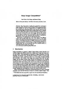
Figure 1: A surface on a uniform grid. practice k 2 proved to be sufficient (using higher values for k did not significantly reduce l a � S � for most surfaces S). At this stage each surface S is registered in all voxels appearing in the list l a � S � . As a result, each voxel in la � S � contains in its surface list an element pointing to S. Thus for each average-sized surface S, we actually obtain a possibly concave and highly tight bounding volume consisting of several small boxes (voxels). This is shown in the two-dimensional example illustrated in Figure 1, where the ordinary bounding box of the surface S is drawn in dashed lines, and the voxels in which it is registered have double boundaries. By using both the bounding box and the set of containing voxels, even tighter bounding volume is obtained: only rays both passing through at least one of the marked voxels and intersecting B � S � are tested further against S. For example, ray A in Figure 1 need not be intersected with S since it does not pass through any of the relevant voxels (although it intersects B � S � ). On the other hand, ray B passes through the right voxels but it will not be intersected with S since it misses B � S � . The bounding box B � S � can be computed by taking the minima and maxima of the B´ezier control points along each of the three dimensions. Such a box, however, is not very tight, since control points could be quite far from the surface they define. We can generally obtain a tighter box by setting B � S ��
�4 �
B � Si �
i 1
where S1 ��������� S4 are the subsurfaces of S over four quarters of the underlying parametric region. These subsurfaces are computed during the computation of l a � S � , and thus the tighter box is obtained at no extra cost. Figure 2 shows a B´ezier curve segment whose control points are marked with bold circles. The bounding box obtained from these control points (drawn with solid lines) contains much void space. After one subdivision, new control points are obtained for the two halves of the curve. These are marked with thin circles. The resulting bounding box (drawn with dashed lines) is much tighter. An even tighter box (drawn with dotted lines) can be obtained after one more subdivision of each of the halves. The scheme described above is most advantageous for “big” surfaces, penetrating a large number of voxels. Note that these are precisely the surfaces for which tight bounding volumes are most necessary, since it is highly probable that many rays will be tested against them during the ray tracing process. Almost no improvement is obtained for surfaces completely contained in a single voxel. For such a surface, however, 7
Figure 2: Using subdivision to obtain a tighter bounding box. a tight bounding volume is less crucial, since only the few rays which happen to pass through its voxel need be tested against it. When a ray passes through several voxels containing the same surface, redundant testing for intersection may arise. To avoid this redundancy we use a mechanism resembling the mailbox mechanism described by Arnaldi et al. [Arna87]. Each ray is assigned a unique integer. Each surface S has a mailbox associated with it that contains the number of the ray most recently tested against B � S � (no matter what the result was). Before testing a current ray against B � S � , we compare the number of this ray with the number in the corresponding mailbox. If these numbers differ, we know that the current ray has not yet been tested against this surface. We register the current ray number in the mailbox and proceed with the test. If the ray intersects the surface, the intersection point is computed (even if it is not inside the current voxel). We maintain a record containing the closest intersection detected so far and the number of the voxel in which it occurs. If the current intersection is closer to the origin, this record is updated accordingly. Thus if the same surface appears again in some subsequent voxel along the path of the ray, the number in its mailbox will match the number of the ray, and the test will not be repeated. Now the complete space tracing scheme can finally be presented: 1. Intersect the ray with the scene bounding box. If there is no intersection, return reporting a miss. 2. Obtain Vfirst and Vlast , the first and the last voxels through which the ray passes. 3. For each nonempty voxel V along the ray, from Vfirst to Vlast do: (a) For each surface S registered in V do: i. If the current ray was the last ray tested against B � S � , continue to the next surface. ii. Update the number of the last ray tested against B � S � . iii. If the ray intersects B � S � , insert S into a list, sorted by the distance from the ray origin. (b) Pass the list to the ray-surface intersection routine described in Section 4. (c) If no intersection was found, continue to the next voxel. (d) Let V be the voxel containing the intersection point. If this intersection is closest to the origin so far, store the parameter values corresponding to this intersection, and set Vlast to V . 8
4 Surface Tree Caching In this section a new algorithm for intersecting rays with parametric surfaces is described. The algorithm is a hybrid between Toth’s algorithm and the subdivision algorithm of Rubin and Whitted. Our algorithm significantly reduces the average cost of intersection calculations, compared to both these methods. Information computed while intersecting each ray is cached, and can later be reused for other rays, thus utilizing ray coherence. To prevent cache overflow, the LRU (least recently used) replacement strategy (see e.g., [Pete85]) is used.
4.1 Mathematical Preliminaries Since our algorithm is based on that of Toth, we begin with a short overview of mathematical background and the results used by Toth. Our purpose is to explain the reasoning behind these results. The reader interested in details and proofs is referred to the original work of Toth [Toth85]. An intersection between a surface s � u � v � and a ray r � t � occurs when and only when s � u � v� � r � t �
f � u � v� t �
0
This nonlinear system can be solved using three-dimensional multivariate Newton iteration. Let x The nonlinear system (1) can now be written in vector form as f � x�
0
�
(1) u � v� t � . (2)
If Y is any 3 � 3 nonsingular matrix, then the Newton scheme is given by xk �
1
xk � Y f � x k �
(3)
The vector � Y f � xk � is referred to as the Newton step. If Y is the inverse Jacobian of f at x k , then xk � 1 , the result of the Newton step, is the point (in parameter space) of intersection between the ray and the tangent plane to the surface at xk . In ordinary Newton iteration, the matrix Y is updated at each step k � 1 to reflect the inverse Jacobian at xk , yielding quadratic convergence. If the matrix Y is held fixed, then Eq. (3) is referred to as simple Newton iteration, yielding only linear convergence. To ensure convergence to the correct solution, a good initial guess is needed. How can this guess be obtained? Let f be a continuously differentiable vector-valued function on the open subset D of threedimensional Euclidian space (the parameter space, in our case), and let X be a box contained in D. For any real vector y in X, and a nonsingular 3 � 3 real matrix Y , an operator K � X � y � Y � referred to as Krawczyk’s operator, can be defined. Krawczyk’s operator provides us with a bound on the movements of elements of X under the Newton step performed with matrix Y : for each x � X, the result of x � Y f � x � is in K � X � y � Y � . Moreover, it can be shown that all solutions in X to system (2) are in K � X � y � Y � . Therefore if K � X � y � Y ��� X 0/ then there are no solutions to system (2) in X. In fact, the result of K � X � y � Y � is another box in parameter space. A solution can exist only where the two boxes overlap. If there is no overlap, there are no solutions in X. Using Krawczyk’s operator Toth defines two criteria for identifying “safe” regions for starting the simple Newton iteration. When a region X in parameter space satisfies one of these criteria, the simple Newton iteration is guaranteed to converge to a single solution for system (2) from any starting point in X.
4.2 The Search for Intersections Using Toth’s safeness criteria, we can present a scheme for finding the ray-surface intersection closest to the ray origin. Given a candidate surface, we compute Krawczyk’s operator and check whether Toth’s criteria 9
are satisfied. If they are, simple Newton iteration is invoked to obtain the solution. Otherwise the surface is regularly subdivided into four subsurfaces. The search for intersections continues only on those subsurfaces whose bounding boxes are hit by the ray, and whose corresponding parametric regions overlap K � X � y � Y � . The main difference between our algorithm and that of Toth’s is that we use regular subdivision, while Toth continues the search after subdividing K � X � y � Y ��� X. This difference may seem insignificant, but we intend to show that our approach enables utilization of ray coherence, which is impossible when using Toth’s algorithm. Before that, however, we present the entire search algorithm in more detail. Given a ray to intersect with the environment, a list L of candidates for intersection is generated. The exact procedure which establishes these candidates depends on the representation of the scene. For instance, the procedure described in Section 3 can be used. u min � umax , V vmin � vmax , and Each element in L is actually a pair � X � S � where X � U � V � T � , U T tmin � tmax . The intervals U and V are the region of parameter space on which the surface S is defined. T is the interval on which the ray parameter t ranges while inside the bounding volume of surface S. The list is sorted on tmin , the approximate distance of each surface from the ray’s origin. This allows closer solutions to be found first. 0. This is done as follows: The elements in L are examined for solutions to f � x �
�
�
�
� �
�
1. While list L is not empty do: 2. Remove the first element from L. Let X 0 be its parametric region. 3. If a solution � u � v� t � has already been found such that t is smaller than t min in X0 , then exit loop; since the list is sorted on tmin , the solution previously found must be the closest to the origin. 4. If the region X0 is too small for analysis, or the portion of surface S corresponding to X 0 is approximately planar, perform a single Newton step. If the step stays in X 0 , consider it a solution, else conclude that there are no solutions in X 0 . Go back to Step 1. 5. Calculate K � X0 � y0 � Y0 � . The choice of y0 and Y0 , and an efficient way of computing K � X 0 � y0 � Y0 � is described in detail by Toth [Toth85]. / then there are no solutions in X0 , and the region can be excluded from 6. If K � X0 � y0 � Y0 � � X0 0, further consideration. Go back to Step 1. 7. If at least one of the two safeness criteria of Toth is satisfied, begin simple Newton iteration to obtain a solution. Store the solution if it is closest to the origin among those found so far. Go back to Step 1. 8. Subdivide X0 regularly into four subregions X1 ��������� X4 (by halving each of the intervals U and V ). Compute bounding boxes for the portions of S corresponding to these subregions. 9. For each of the subregions do: If the subregion overlaps K � X 0 � y0 � Y0 � (i.e., a solution there is possible), intersect the ray with the corresponding bounding box. If there is no overlap, or if the ray misses the bounding box, the corresponding subregion is excluded from further search. Create list elements for subregions whose bounding boxes were intersected, and insert them into the list L preserving its order. Go back to Step 1. In Toth’s algorithm, instead of subdividing X 0 , K � X0 � y0 � Y0 ��� X0 is subdivided into two subregions X 1 and X2 . The search process for each surface, corresponds to a binary tree over the underlying parametric region. The root of this tree is associated with the entire region on which the search begins (e.g., 0 � 1 � 0 � 1 ). If a region X0 was excluded or if Newton iteration began there, then a node associated with this region is a leaf node. Otherwise, it is an internal node having nodes associated with X 1 and X2 as its children. An
�
�
10
V 1 A A
B D
E
B
C
C
D 0
1
E
U
(a)
(b)
Figure 3: A possible search in parameter space (a) and the corresponding binary tree (b). example of a tree resulting from a possible search process is illustrated in Figure 3. The boxes drawn with dashed lines correspond to values of Krawczyk’s operator, calculated for the parametric regions A and B. For each ray, the entire search process is repeated several times from scratch (once for each candidate surface). Can we reduce the amount of computation by actually constructing the corresponding trees, caching them and later reusing them for other rays? The parametric subregions of each node in such a tree are determined by both the surface and the current ray, since the value of Krawczyk’s operator depends on the direction of the ray. Therefore, two different rays will generally produce two different trees for the same surface. This is true even if both rays strike the surface at the same point. It seems that reusage of computed information in Toth’s method is difficult. When our algorithm is used, the search process corresponds to a quadtree over the parametric region underlying the surface. We refer to such trees as “surface trees”. An example of a possible surface tree is illustrated in Figure 4. Surface trees may develop differently for different rays, but they all subdivide the parametric region in the same regular fashion. Now suppose that, while intersecting a surface by a ray for the first time, we actually construct a surface tree corresponding to the search process. After this search ends the tree will be cached. Associated with each node are the appropriate parametric subregion and a bounding box for the surface over this subregion. The next time a ray is tested against this surface, it is first intersected with the cached surface tree. Only the parametric subregions corresponding to those leaves whose bounding boxes are intersected by the ray need be searched for intersection. In many cases it turns out that the ray misses all the leaves, and no further search is necessary for that surface. In the remaining cases the number of required search iterations will be small, since they begin on small parametric subregions. When a ray is tested against a surface for which no tree is cached yet, the search begins from the complete parametric region. In this case probably more search iterations will be needed, compared to Toth’s search scheme. Most of the rays, however, succeed in reusing previously computed information, and the average number of search iterations per ray is considerably lower in our algorithm. Since each search iteration is rather expensive, substantial computational savings are obtained by reducing the number of these iterations. Furthermore, in our algorithm, in each iteration a patch is split into four. In Toth’s algorithm first a subpatch is calculated, and then the subpatch is split in two. This requires more floating point operations than splitting a patch into four. Thus each search iteration in our algorithm is also cheaper than in Toth’s. Timing results are given in Section 7.
11
V 1 A
D
E
F
G A
B
B
C
C
D
0
1
E
F
G
U
(a)
(b)
Figure 4: A possible search in parameter space (a) and the corresponding quadtree (b). As was mentioned before, our algorithm is a hybrid between Toth’s algorithm and the subdivision algorithm of Rubin and Whitted, which also constructs and caches surface trees. The advantages of our approach over Toth’s have already been explained. Now we explain why our approach is better than the pure subdivision approach of Rubin and Whitted. In their method, the search for intersection is guided entirely by the results of intersecting the ray with bounding volumes. We utilize an additional tool: Krawczyk’s operator. We use it to exclude parametric regions, and to identify regions in which convergence of simple Newton iteration is guaranteed. Typically, when constructing a surface tree, only a small number of subdivisions need be performed, before the entire surface is excluded, or a safe region is identified. Thus the cost associated with construction of surface trees is considerably smaller when our algorithm is used. The resulting surface trees are less deep. Less storage is required for them, and less ray-box intersections need be performed, to locate the intersected leaves in each tree. Thus, reusage of cached information is also cheaper in our algorithm.
4.3 Cache Size Control Naturally, the size of the cache must be limited. Whenever the cached surface trees take up too much space, we have to free some of them in order to make room for newly created trees. The question arises: What trees should be released from the cache? To answer this question we use a version of the well-known LRU algorithm. This is a page replacement algorithm used in operating systems for virtual memory management [Pete85]. We maintain a queue that is implemented as a doubly linked list. Elements in this queue point to the roots of cached trees. Each time a surface is tested against a ray, its tree is inserted at the end of the queue. If this tree was already in the queue it is removed first. Thus, the first element in the queue always points to the tree which was least recently used by any ray. Therefore, whenever the need arises, trees are released from the head of the queue. To see why LRU is indeed a successful choice, note the analogies between our caching scheme and paging in virtual memory. The surfaces tested against a particular ray correspond to memory references resulting from execution of a machine instruction. When no tree is cached for some tested surface this
12
corresponds to a page fault. Both cache miss and page fault result in time penalty: recomputing the surface tree and loading the required page from secondary storage. LRU was found to be a successful paging algorithm due to the locality of reference property exhibited by fragments of computer programs. In our case the analog for that property is ray coherence. Adjacent ray trees tend to intersect the same set of surfaces, just like adjacent instructions tend to reference the same areas in address space.
5 Better Sampling Orders In standard ray tracing, the order in which the image space is sampled has no significance. Normally, in sequential software implementations the image space is sampled in scanline order. However, when ray coherence is utilized, a smarter sampling strategy may result in speedier execution. Eye rays can be classified into coherence groups. Each coherence group corresponds to a coherent area of the image plane (i.e., an area through which the same surface is visible). Secondary rays spawned by eye rays of the same coherence group are also likely to be coherent. In general, the deeper the rays are in the ray tree, the weaker the coherence between them. This is especially true in distributed ray tracing, in which directions of rays are randomly jittered. When the image plane is sampled in scan line order, eye rays belonging to the same coherence group are generally generated in several disjoint spans. At least one such span exists for each scan line, where it crosses the projection of the visible surface on the image plane. Between these spans, cached information corresponding to this surface is usually lost, being replaced by more recently computed information. Thus, at the beginning of each span the necessary information is recomputed from scratch. We are therefore interested in finding a sampling order which will minimize the number of these disjoint spans for each coherence group. In this section two sampling orders are described which attempt to achieve this minimization. A quantitative comparison between these two orders is given in Section 7.
5.1 The Item Buffer Order The concept of item buffer was introduced by Weghorst et al. [Wegh84]. Originally it was used to speed up the search for surfaces intersected by eye rays. As a preprocess to ray tracing, a visible surface algorithm (e.g., z-buffer) is invoked with the same viewing parameters. Instead of producing an ordinary display buffer with intensity values for each pixel in the image, the visible surface algorithm produces an item buffer. Each entry within the item buffer (corresponding to a small area of the image plane) contains the list of surfaces visible through that area. In most entries, for a typical image, these lists contain a single element, or they are empty. Normally, for each eye ray, the item buffer provides the ray tracer with a short list of candidates for intersection. Thus, much of the computational effort invested in tracing eye rays is saved. In the case of parametric surfaces, the approach described here yields less significant savings. In the case of parametric surfaces most of the time is spent on the calculation of the intersection point. This time is not eliminated by the ordinary item buffer technique. Relatively little time is spent on determining the candidates for intersection, and the uniform subdivision (which is an extension of the item buffer to three dimensions) does a satisfactory job of that. We feel that the item buffer can be used with parametric surfaces if each item also contains the parametric values corresponding to the portion of surface visible through its pixel. In this work we propose another use for the item buffer: it can provide a better order for image space sampling. From the item buffer we can obtain for each surface the pixels through which it is visible. Thus, we are able to trace all the eye rays corresponding to these pixels consecutively. The problems with this approach are: (i) a very robust visible surface processor for parametric surfaces is needed and (ii) the full resolution item buffer significantly increases the memory requirements of the rendering process. 13
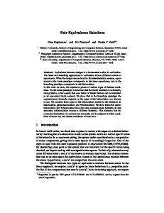
Figure 5: A Peano curve covering a 16 � 16 grid. To overcome these problems an approximation is used. Instead of generating a full resolution exact item buffer, a low resolution (e.g., 64 � 64) buffer is produced. In each entry only one surface can be registered. Among all the surfaces whose projections of the bounding boxes overlap the area corresponding to the entry, the closest is chosen. The resulting inaccuracies can cause no harm, since the buffer is only used to produce a better sampling order; this information is not used by the intersection process. Thus, at the cost of a less accurate sampling order, the need in a visible surface processor and a large memory is eliminated.
5.2 The Peano Curve Order Peano curves are recursive space-filling curves. These curves have a property which makes them attractive for use in image processing and computer graphics (see, e.g., [Witt82]). Observe the example of a Peano curve covering a 16 � 16 grid in Figure 5. Examination of the path shows that if the image is divided into four quadrants, all the points in any one of them are visited by the Peano curve before it proceeds to the next. Furthermore, the same result is obtained when a quadrant is recursively subdivided into four more, and so on. Therefore, sampling the pixels on the image plane in the order they are visited by a Peano curve seems promising. The clusters of successively sampled pixels are now two-dimensional, rather than onedimensional (in scan line order). Eye rays belonging to the same coherence group are no longer generated in many disjoint spans. Another advantage of the Peano curve sampling order is that it is very easy to implement, compared to the item buffer order. A recursive routine generating pixels in Peano curve order takes but a few lines of code. The depth of recursion is only logarithmic in the resolution of the image. No extra memory or preprocessing is required.
6 Improved Treatment of Secondary Rays In a typical ray-traced image much of the computational effort is invested in tracing secondary (i.e., reflected, refracted and shadow) rays. This effort becomes larger when the scene contains more highly reflective and transparent surfaces or more light sources. The main difference between secondary rays and primary (eye) rays is that secondary rays intersect at least one surface in the scene — the surface of origin. The ray
14
parameter corresponding to this trivial intersection is 0 (but due to numerical inaccuracies it may actually be somewhere between � δ and � δ, where δ is a small number that depends on the average size of the objects and the overall scale). Hence, when tracing secondary rays we are interested not in the solution closest to the origin, but in the next closest solution. When the secondary ray emerges from a convex surface (e.g., a polygonal facet), we can simply exclude this surface from the intersection search for that ray. When parametric surfaces of higher than linear degree are ray-traced, however, no such exclusion can be made. The ray may have a nontrivial intersection point with the surface of its origin in case of self-shadowing or self-reflection. Thus, for each secondary ray, hundreds of floating point operations may be wasted on trivial intersections. This problem has been ignored in all the methods described in Section 2. In this section we propose modifications to the algorithm presented in Section 4 that can significantly reduce the amount of computation wasted on trivial intersections. These modifications can also be applied to Toth’s original intersection algorithm. Recall the search loop in Section 4.2. The search takes place in parameter space. The candidate parametric subregions (corresponding to subsurfaces of the original surfaces) are kept in a sorted list. For each subregion the corresponding interval of the ray parameter t min � tmax is kept. All the intersections (if any) between the ray and the corresponding subsurface must occur within this interval. Therefore, if the subregion in question belongs to the surface of origin, and t max δ, we may safely exclude this subregion from further consideration. This can be done because every solution found there will be identified as trivial. A similar test can be performed again, after Krawczyk’s operator has been computed. Recall that Krawczyk’s operator provides us with bounds on the parametric values of the possible solutions in the current parametric subregion. Again, if the subregion belongs to the surface of origin, and the upper bound given by Krawczyk’s operator on the value of t is smaller than δ, the subregion can be excluded. Next, Toth’s safeness criteria are evaluated. If at least one of these is satisfied, then there is a single solution in the current subregion. Therefore, if the subregion corresponds to the surface of origin, and the lower bound tmin on the ray parameter satisfies tmin 0, then this solution must be trivial. In this case, again, the subregion can be dropped. By introducing these three “triviality tests” into the search loop, parametric subregions containing trivial intersections are identified before these intersections are found and calculated. A certain amount of needless computation is thus saved for almost every secondary ray. When the caching scheme described in Section 4 is used, these subregions are usually identified at the beginning of the first search iteration, and the wasted computation is minimized. In the particular case of shadow rays, further savings can be obtained. One algorithm for efficient handling of shadow rays was already described by Haines and Greenberg [Hain84]. We describe some additional savings that are possible when ray tracing parametric surfaces. The purpose of a shadow ray is to determine whether a light source is visible from a given point on a surface. We may stop tracing a shadow ray the moment we are sure that it intersects some opaque surface that is closer to its origin than the light source. The exact intersection point is of no interest to us in this case, since it is only the existence of the intersection that matters. The conclusion is that another improvement can be introduced into the intersection algorithm. When any of the safeness criteria is satisfied, simple Newton iteration is guaranteed to converge to a solution. If the current ray is a shadow ray, and the intersected surface is opaque, the intersection routine may return at that point, reporting that intersection has occurred. Thus the simple Newton iteration is not entered at all. Note that this improvement is not possible in other methods mentioned in Section 2, since in those methods no criteria exist that guarantee convergence.
�
�
15
num. of objects num. of patches num. of lights max. ray tree depth num. of voxels percent nonempty voxels surfaces per nonempty voxel resolution total num. of rays rays that hit av. ray tree depth non-cache memory cache size
Test 1 1 32 1 5 630 36.98 2.20 512 482994 319616 2.18 20692 500K
Test 2 50 1600 1 1 24360 12.54 3.95 512 437452 351241 1 635384 1000K
Test 3 50 1600 1 5 24360 12.54 3.95 512 773479 687264 2.57 635384 1000K
Test 4 50 1600 6 5 24360 12.54 3.95 512 1934605 1848349 2.57 635384 1000K
Test 5 100 3200 1 5 26100 18.64 4.26 512 925193 868131 2.78 1499840 500K
Table 1: Specifications for the test cases.
7 Results The improved method for ray tracing parametric surfaces, based on the techniques presented in the previous sections, was implemented as part of the Hebrew University Ray Tracing Package. The ray tracing package was implemented in the C programming language and installed on several different machines, ranging from workstations to a mainframe. In order to demonstrate the computational efficiency of the proposed techniques, various test environments have been modeled and rendered. These environments differ in the number of objects, their size relative to the size of the image, number of light sources, and in the maximum depth of the ray trees. In this section we describe these tests, present their results, and discuss them.
7.1 Timing Tests In each timing test a test environment was rendered five times: 1. Using ordinary Toth’s method (TOTH). 2. Using Toth’s method enhanced with improved handling of secondary rays (ISRT). 3. Using the tree caching method with scan line sampling (SCAN). 4. Using the tree caching method with an approximate 64 � 64 item buffer (ITBUF). 5. Using the tree caching method with Peano curve order sampling (PEANO). The uniform spatial subdivision technique described in Section 3 was used in all cases above. Although no special timing test was devised to measure the effectiveness of uniform spatial subdivision, it is demonstrated by measuring the number of surfaces tested against each ray. The specifications for all tests are given in Table 1. The test environments are constructed exclusively from Utah teapots. Each teapot is modeled with 32 bicubic B´ezier patches. Teapots were chosen because of their complex shapes, demonstrating a variety of curvatures, coinciding control vertices, and intersecting surfaces. The control vertices data was taken from [Crow87]. In each timing test the following processing statistics were measured and reported: 16
Normalized time The total cpu time required for ray tracing. This includes everything except the time required for initialization (less than 1 percent of the total time in all renderings). Times are normalized such that the time for ordinary Toth’s method is 1.0. Surfaces tested per ray The average number of surfaces per ray whose outmost bounding boxes were tested (to demonstrate the effectiveness of the uniform spatial subdivision scheme). Only rays hitting the bounding box of the entire environment were counted. Surfaces searched per ray The average number of surfaces per ray which entered the search loop (to demonstrate the effectiveness of the surface trees scheme). Only rays hitting the bounding box of the entire environment were counted. Ray-box tests per ray The average number of ray-box intersection calculations per ray. All rays were counted. Search iterations per ray The average number of search iterations per ray. Only rays hitting the bounding box of the entire environment were counted. Newton starts per ray The average number of times simple Newton iteration was initiated per ray. Only rays hitting some surface in the environment were counted. Average safe region width The average width of the parametric regions in which simple Newton iterations was initiated. Simple Newton iterations per call The average number of simple Newton iterations per call. Cache misses per surface The average number of times each surface was tested without precomputed information. Cache hit ratio The percent of ray-surface tests in which cached information was used. The timing tests were performed on all the machines on which the package was installed. This was done to ensure that acceleration is obtained with our improved method, regardless of the machine used. Indeed, the acceleration and the other statistics measured were approximately the same for all machines. The statistics reported in this section were all measured on a 4-Mbyte SUN 3/110 workstation with Motorola MC68881 floating point processor and without floating point accelerator. All floating point calculations were performed in single precision. We do not give absolute cpu times, since these are often misleading, being too dependent on programming style, code optimization, and hardware. The number of flops per ray is also not very meaningful in this case because it tends to vary drastically from scene to scene, and even from ray to ray in the same scene, hitting the same surface. Both the time and the number of flops are strongly influenced by the size of the cache, and the resolution of the spatial subdivision, which in turn are a function of the total amount of available memory and the size of the data base. By our timing tests we are not trying to prove that our method is the fastest. Rather, we attempt to demonstrate the effectiveness of the techniques employed. We feel that the statistics that we report are adequate for this purpose.
7.2 Discussion of Results In the first timing test, an environment including a single large reflective teapot was rendered. The image is shown in Figure 6. The processing statistics are concentrated in Table 2. It can be seen that improved 17
Figure 6: The pink teapot. handling of secondary rays results in a significant reduction in the number of search iterations required per ray. The number of times that Newton iteration had to be initiated is also considerably smaller. This is because trivial intersections and occluding surfaces are identified before the exact intersection is found. The technique introduces a 10 percent reduction in total execution time. As expected, the tree caching scheme has proven to be very effective, reducing the total execution time by a factor of four. Note that the number of surfaces whose bounding box is tested against each ray is approximately the same in all cases. However, the number of surfaces actually searched for solutions is significantly smaller when the tree caching scheme employed. Many rays that intersect the bounding box of a surface miss all the leaves of the cached surface tree. Therefore, many additional surfaces can be excluded from the search for intersections. The number of search iterations performed per ray is also drastically reduced, because the search begins from small parametric subregions for each surface. The number of the ray-box intersection calculations is larger, but this increase is outweighed by the reductions mentioned earlier. Sampling in item buffer order and in Peano curve order results in a total execution time 8 percent smaller than in the scan line case. Note also the decrease in cache misses, and the increase in cache hit ratio obtained with these sampling orders. The next test environment (Table 3) includes 50 non-reflective teapots. The teapots were randomly scattered in the environment. The results are very similar to those obtained in the first test, although this environment is far less coherent, compared to the previous one. Note the effectiveness of the combined spatial subdivision and surface trees approach: although there are 1600 patches in the environment, only 6.82 surface trees are tested against each ray (due to the spatial subdivision scheme). Among these only 1.27 surfaces are searched for intersections (due to the surface trees). In the third test (Figure 7, Table 4) the same environment as before was used. This time the teapots were defined as reflective. As a result, the number of traced rays is almost twice as high. The additional rays are all secondary rays for which ray coherence is typically weaker. Even so, similar improvement is observed. This time the improvement obtained by better sampling orders is more significant. Since in this test many 18
normalized time surfaces tested / ray surfaces searched / ray ray-box tests / ray search iterations / ray Newton starts / ray Newton iterations / call av. width of safe regions cache misses / surface cache hit ratio
TOTH 1.00 3.04 2.11 18.30 7.42 1.05 1.36 0.134
ISRT 0.90 3.02 2.10 17.52 6.68 0.37 1.44 0.155
SCAN 0.26 3.02 1.06 42.12 2.82 0.37 1.08 0.027 104.72 99.00
ITBUF 0.24 3.02 1.04 44.23 2.59 0.37 1.07 0.026 66.59 99.35
PEANO 0.24 3.02 1.03 44.84 2.56 0.37 1.06 0.025 59.84 99.39
Table 2: Processing statistics for test case 1.
normalized time surfaces tested / ray surfaces searched / ray ray-box tests / ray search iterations / ray Newton starts / ray Newton iterations / call av. width of safe regions cache misses / surface cache hit ratio
TOTH 1.00 6.88 2.81 27.68 7.62 1.02 1.37 0.146
ISRT 0.93 6.81 2.78 26.88 7.10 0.50 1.38 0.150
SCAN 0.30 6.82 1.33 54.69 2.93 0.51 1.14 0.041 6.16 94.59
ITBUF 0.29 6.82 1.27 57.04 2.72 0.51 1.12 0.040 1.95 96.74
PEANO 0.29 6.82 1.27 57.40 2.73 0.51 1.11 0.036 1.13 96.93
Table 3: Processing statistics for test case 2.
normalized time surfaces tested / ray surfaces searched / ray ray-box tests / ray search iterations / ray Newton starts / ray Newton iterations / call av. width of safe regions cache misses / surface cache hit ratio
TOTH 1.00 8.42 3.62 36.81 11.06 1.17 1.32 0.128
ISRT 0.91 8.35 3.58 35.59 10.20 0.41 1.34 0.135
SCAN 0.35 8.36 1.96 61.95 5.31 0.42 1.27 0.061 117.98 84.50
ITBUF 0.30 8.36 1.72 70.18 4.50 0.42 1.21 0.051 72.20 88.97
Table 4: Processing statistics for test case 3.
19
PEANO 0.29 8.36 1.71 70.99 4.47 0.42 1.19 0.048 68.42 89.42
Figure 7: 50 flying teapots. secondary rays were involved, sampling orders which result in more coherent rays are especially important. It can be observed that performance of Peano order is somewhat better than item buffer order. The same environment was rendered again with six light sources (Table 5). Due to the larger portion of shadow rays, improved treatment of secondary rays yields more significant reduction of execution time than in the other cases. Note the very small Newton starts per ray ratio. The last test environment (Figure 8, Table 6) includes 100 reflective teapots. Although the number of surfaces is doubled, and the image is less coherent, our method is still almost three times quicker than Toth’s. There is an undesirable tendency that can be observed in all timing tests. The safe regions decrease in width when coherence is exploited. This means that when many coherent rays are traced the surface trees tend to grow deeper. As a result, more time has to be spent while intersecting each ray with these trees. Another consequence of this is that the cache fills up quickly, so that only a small number of recently used surface trees is cached at each moment. The conclusion is that this growth must be limited. Branches beyond certain depth should not be cached.
8 Conclusions In this work, a new method for ray tracing parametric surfaces has been presented. A uniform spatial subdivision scheme to handle parametric surfaces has been adapted to handle parametric surfaces. The spatial subdivision is coupled with hierarchies of bounding boxes (surface trees) to cull surfaces from performing intersection calculations with a ray. A new intersection algorithm, which allows dynamic and adaptive generation of surface trees, was developed. The surface trees are cached for later reusage by other rays, thus utilizing ray coherence. An LRU (least recently used) algorithm is employed to select surface trees for release from the cache when it fills up. Utilization of ray coherence is facilitated by sampling the image space in new nonconventional orders: item buffer order, based on visible surfaces preprocessing, and Peano curve order. Improvements which allow computational savings when tracing secondary rays have also been
20
normalized time surfaces tested / ray surfaces searched / ray ray-box tests / ray search iterations / ray Newton starts / ray Newton iterations / call av. width of safe regions cache misses / surface cache hit ratio
TOTH 1.00 8.37 3.54 37.32 11.45 1.15 1.33 0.131
ISRT 0.88 8.17 3.45 35.33 10.20 0.15 1.34 0.135
SCAN 0.28 8.20 1.75 63.77 4.90 0.16 1.27 0.062 159.17 90.72
ITBUF 0.26 8.20 1.58 71.60 4.25 0.15 1.20 0.050 107.47 92.90
PEANO 0.26 8.20 1.58 72.29 4.24 0.15 1.19 0.048 102.77 93.14
Table 5: Processing statistics for test case 4.
normalized time surfaces tested / ray surfaces searched / ray ray-box tests / ray search iterations / ray Newton starts / ray Newton iterations / call av. width of safe regions cache misses / surface cache hit ratio
TOTH 1.00 10.67 4.14 42.39 12.29 1.24 1.32 0.124
ISRT 0.91 10.56 4.10 40.96 11.31 0.43 1.33 0.129
SCAN 0.40 10.57 2.43 66.12 6.48 0.44 1.33 0.070 154.38 74.46
ITBUF 0.36 10.57 2.19 73.63 5.65 0.44 1.27 0.061 115.93 78.63
Table 6: Processing statistics for test case 5.
21
PEANO 0.35 10.57 2.18 74.41 5.62 0.44 1.26 0.058 111.47 79.22
Figure 8: 100 flying teapots. presented. The new method was implemented, and various images were rendered using it, on several hardware platforms, among these a 4 Mbyte workstation. Statistics for various test environments that differ in the number of objects, number of light sources, and the reflective properties of the objects consistently indicate substantial improvement of the new method over Toth’s method. Although some of the other methods mentioned in Section 2 may be faster than our method, ours is qualitatively superior to them, since it does not possess their disadvantages. Further research is required on a number of topics. It should be investigated whether using the exact item buffer, rather than the approximate one, will lead to better sampling order than the Peano curve order. Ways to exploit the item buffer for speeding up the intersection calculations of eye rays is another issue. Smarter control of depth for surface trees should lead to further improvements of our method: the cache will fill up more slowly, and the utilization of coherence will be more fruitful. Another possible improvement to the surface tree caching scheme involves a more sophisticated strategy for releasing cached surface trees. Instead of releasing an entire tree we might prune several trees.
References [Appe68] Appel, Arthur, ”Some Techniques for Shading Machine Renderings of Solids”, AFIPS 1968 Spring Joint Computer Conference, vol. 32, 1968, pp. 37–45. [Arna87] Arnaldi, Bruno, Thierry Priol, Kadi Bouatouch, ”A New Space Subdivision Method for Ray Tracing CSG Modelled Scenes”, The Visual Computer, Springer-Verlag, vol. 3, no. 2, Aug. 1987, pp. 98–108. [Clea88] Cleary, John G., Geoff Wyvil, “An Analysis of an Algorithm for Fast Ray-Tracing using Uniform Space Subdivision”, The Visual Computer, Springer-Verlag, vol. 4, no. 2, July 1988, pp. 65–83.
22
[Cook84] Cook, Robert L., Thomas Porter, Loren Carpenter, “Distributed Ray Tracing”, Computer Graphics (SIGGRAPH ’84 Proceedings), vol. 18, no. 3, July 1984, pp. 137–145. [Crow87] Crow, Frank, “The Origins of the Teapot”, IEEE Computer Graphics and Applications, vol. 7, no. 1, Jan. 1987, pp. 8–19. [Fuji86] Fujimoto, Akira, Takayuki Tanaka, Kansei Iwata, “ARTS: Accelerated Ray-Tracing System”, IEEE Computer Graphics and Applications, vol. 6, no. 4, Apr. 1986, pp. 16–26. [Glas84] Glassner, Andrew S., “Space Subdivision for Fast Ray Tracing”, IEEE Computer Graphics and Applications, vol. 4, no. 10, Oct. 1984, pp. 15–22. [Glas88] Glassner, Andrew S., “Spacetime Ray Tracing for Animation”, IEEE Computer Graphics and Applications, vol. 8, no. 2, March 1988, pp. 60–70. [Hain84] Haines Eric A., Donald P. Greenberg, “The Light Buffer: A Ray Tracer Shadow Accelerator”, IEEE Computer Graphics and Applications, vol. 6, no. 9, Sept. 1986, pp. 6–16. [Joy86] Joy, Kenneth I., Murthy N. Bhetanabhotla, “Ray Tracing Parametric Surface Patches Utilizing Numerical Techniques and Ray Coherence”, Computer Graphics (SIGGRAPH ’86 Proceedings), vol. 20, no. 4, Aug. 1986, pp. 279–285. [Kay86] Kay, Timothy L., James T. Kajiya, “Ray Tracing Complex Scenes”, Computer Graphics (SIGGRAPH ’86 Proceedings), vol. 20, no. 4, Aug. 1986, pp. 269–278. [Kaji82] Kajiya, James T., “Ray Tracing Parametric Patches”, Computer Graphics (SIGGRAPH ’82 Proceedings), vol. 16, no. 3, July 1982, pp. 245–254. [Kaji83] Kajiya, James T., “New Techniques for Ray Tracing Procedurally Defined Objects”, ACM Transactions on Graphics, vol. 2, no. 3, July 1983, pp. 161–181. [Kapl85] Kaplan, Michael R., “Space Tracing, A Constant Time Ray-Tracer”, SIGGRAPH ’85 State of the Art in Image Synthesis seminar notes, July 1985. [Levn87] Levner, Geoff, Paolo Tassinari, Daniele Marini, “A Simple Method for Ray Tracing Bicubic Surfaces”, Computer Graphics 1987, Tosiyasu L. Kunii ed., Springer-Verlag, Tokyo, 1987, pp. 285– 302. [Math68] Mathematical Applications Group Inc., “3-D Simulated Graphics”, Datamation, Feb. 1968. [Pete85] Peterson James L., Abraham Silberschatz, Operating System Concepts, Addison-Wesley, Reading, Massachusets, 1985. [Pull87] Pulleyblank, Ron, John Capenga, “The Feasibility of a VLSI Chip for Ray Tracing Bicubic Patches”, IEEE Computer Graphics and Applications, vol. 7, no. 3, March 1987, pp. 33–44. [Ries80] Riesenfeld, Richard, Elaine Cohen, Tom Lyche, “Discrete B-Splines and Subdivision Techniques in Computer-Aided Geometric Design and Computer Graphics”, Computer Graphics and Image Processing, vol. 14, no. 2, Oct. 1980, pp. 87–111. [Rubi80] Rubin, Steven M., Turner Whitted, “A 3-Dimensional Representation for Fast Rendering of Complex Scenes”, Computer Graphics (SIGGRAPH ’80 Proceedings), vol. 14, no. 3, July 1980, pp. 110– 116. 23
[Sede83] Sederberg Thomas W., “Implicit and Parametric Curves and Surfaces for Computer Aided Geometric Design”, Ph.D. Thesis, Purdue University, 1983. [Swee86] Sweeney, Michael, Richard H. Bartels, “Ray Tracing Free-Form B-Spline Surfaces”, IEEE Computer Graphics and Applications, vol. 6, no. 2, Feb. 1986, pp. 41–49. [Toth85] Toth, Daniel L., “On Ray Tracing Parametric Surfaces”, Computer Graphics (SIGGRAPH ’85 Proceedings), vol. 19, no. 3, July 1985, pp. 171–179. [Wegh84] Weghorst, Hank, Gary Hooper, Donald P. Greenberg, “Improved Computational Methods for Ray Tracing”, ACM Transactions on Graphics, vol. 3, no. 1, Jan. 1984, pp. 52–69. [Witt82] Witten, Ian H., Radford M. Neal, “Using Peano Curves for Bilevel Display of Continuous-Tone Images”, IEEE Computer Graphics and Applications, vol. 2, no. 3, May 1982, pp. 47–52. [Whit80] Whitted, Turner, “An Improved Illumination Model for Shaded Display”, Communications of the ACM, vol. 23, no. 6, June 1980, pp. 343–349. [Wood89] Woodward, Charles, “Ray Tracing Parametric Surfaces by Subdivision in Viewing Plane”, Proc. Theory and Practice of Geometric Modeling, W. Strasser ed., Springer-Verlag, 1989. [Yang87] Yang, Chang-Gui, “On Speeding Up Ray Tracing of B-Spline Surfaces”, Computer Aided Design, vol. 19, no. 3, April 1987, pp. 122–130.
24