Dec 18, 2009 - Improvement of computer simulation models for metallic melts via quasielastic neutron scattering: A case study of liquid titanium. J. Horbach,1 ...
PHYSICAL REVIEW B 80, 212203 共2009兲
Improvement of computer simulation models for metallic melts via quasielastic neutron scattering: A case study of liquid titanium J. Horbach,1 R. E. Rozas,1 T. Unruh,2 and A. Meyer1 1
Institut für Materialphysik im Weltraum, Deutsches Zentrum für Luft- und Raumfahrt (DLR), 51170 Köln, Germany Forschungsneutronenquelle Heinz Maier-Leibnitz, FRM II, Technische Universität München, 85747 Garching, Germany 共Received 24 November 2009; published 18 December 2009兲
2
A combination of quasielastic neutron scattering 共QNS兲 and molecular-dynamics 共MD兲 simulation is used to modify an embedded atom method 共EAM兲 potential for Ti with respect to the description of melt properties and crystallization from the melt. In the MD simulation, the EAM model is optimized such that agreement with accurate data of self-diffusion coefficients from QNS is achieved. As a result the density and the melting temperature are in good agreement with experiment. DOI: 10.1103/PhysRevB.80.212203
PACS number共s兲: 61.20.Lc, 02.70.Ns, 61.05.F⫺, 61.20.Ja
I. INTRODUCTION
The investigation of metallic liquids and their crystallization from the melt provides a great challenge to experiment and modeling.1,2 Metallic systems typically solidify in a temperature range between 1000 and 2000 K where it is elaborate to carry out experiments on the structure and dynamics of the melt as well as the crystallization process. The modeling of metallic melts via particle-based simulation techniques such as molecular dynamics 共MD兲 suffers from the small experimental database. For this reason, most of the model potentials, that have been developed to describe the effective interactions between the atoms in a metal, have been parameterized with respect to properties of crystalline phases. These potentials often reproduce reliably on a qualitative level various melt properties, such as, e.g., different aspects of transport and structural relaxation.3–6 However, they show systematic quantitative deviations with respect to the temperature dependence of density, structural quantities, mass transport coefficients, and the value of the melting temperature.7–12 In this Brief Report, we show for the example of liquid Ti how an existing potential can be improved using quasielastic neutron-scattering 共QNS兲 data as a reference. The potential, considered here, has been proposed by Zope and Mishin13 共in the following referred to as ZoM model兲. This potential has been fitted to various zero-temperature properties of ␣-Ti 共hcp phase兲 that were obtained from ab initio calculations. Zope and Mishin have shown that it leads to a good agreement with experiment with respect to the high-temperature bcc phase of Ti 共-Ti兲.13 Below we present a simple strategy how one can modify the ZoM model 共and possibly similar model potentials for metals兲 to describe various properties of the melt more accurately, including the location of the melting transition. The basis are accurate measurements of the temperature dependence of the self-diffusion coefficient of the melt. The present work combines state-of-the-art QNS experiments with MD simulation. We demonstrate that the temperature dependence of the self-diffusion coefficient, DTi, is an appropriate feature to adjust an effective potential to experimental data. As a basis for that, a model potential is required that already describes correctly certain trends of the 1098-0121/2009/80共21兲/212203共4兲
materials properties. Then, the QNS data can be used to calibrate the temperature scale of the potential 共see below兲. Realistic potentials for MD simulations are an important requirement for the study of solidification processes in metallic melts. In particular, interfacial properties such as interfacial free energies are in general not accessible from experiments nor from ab initio simulations 共due to the limitation of system size and time scale兲. In MD simulations with effective potentials, such properties can be calculated1,12 and thus, they are a very valuable tool toward a microscopic understanding of crystal growth and nucleation in metallic melts. II. MODIFICATION OF THE POTENTIAL
The aforementioned ZoM potential has been derived in the framework of the embedded atom method 共EAM兲.14 In this framework, one introduces an embedding function Fi共h,i兲 that depends on the host electron density h,i at atom i. The function Fi describes the energy to embed an atom i into the local electron gas due to the other atoms in the system. It is assumed that the host electron density h,i at atom i can be approximated by a linear superposition of pairwise contributions that depend on the distance rij = 兩rជi − rជ j兩 between atoms i and j at positions rជi and rជ j, respectively. The total EAM energy of the system, V, is given by the contributions F共h,i兲 and additional pair interaction terms u共rij兲 that describe the short-ranged hard-core repulsion between N N the atoms, V = 兺i=1 F共h,i兲 + 21 兺i=1 兺Nj⫽iu共rij兲 共with N the total number of atoms in the system兲. The details of the ZoM potential for Ti can be found in the original publication.13 In order to improve the ZoM potential, we multiply the whole EAM potential by a constant ␣ such that the new EAM energy V⬘ is related to the old one by V⬘ = ␣V. As an optimal value for ␣, we found ␣ = 1.245 共in the following we refer to the corresponding modified potential as the ModZoM potential兲. This value was determined by performing MD simulations with different values of ␣ and choosing the value that leads to the best agreement with the self-diffusion data, as obtained by QNS. As we shall see below, the introduction of the parameter ␣ yields essentially an adjustment of the temperature scale, keeping, e.g., properties unchanged that are defined relative to the melting temperature such as crystal-growth coefficients.
212203-1
©2009 The American Physical Society
PHYSICAL REVIEW B 80, 212203 共2009兲
BRIEF REPORTS III. EXPERIMENTAL TECHNIQUES
40
f共q,t兲 = aq exp共− t/q兲
共1兲
with aq an amplitude and q a relaxation time, both depending on wave number q. In the hydrodynamic regime, DTi is related to the relaxation time by 1 / q = DTiq2. We have employed this formula to extract DTi from the QNS data, as shown below.
30 20 vI (m/s)
QNS in combination with electromagnetic levitation has been recently established for the investigation of the dynamics of metallic melts.15 Using these techniques, self-diffusion coefficients can be determined with high accuracy, provided that at low wave numbers q the total scattering signal is dominated by incoherent-scattering contributions. The latter requirement is fulfilled in metallic melts containing, e.g., Ni, Co, or Ti. So far, QNS on levitated samples has been, in particular, used to measure the self-diffusion coefficients of Ni in pure Ni,15 Zr-Ni,16,17 and silicon-rich Si-Ni.18 The QNS measurement of the self-diffusion constant of Ti, DTi, was performed at the neutron time-of-flight spectrometer TOFTOF 共Ref. 19兲 of the FRM II. An electromagnetic levitation device, especially designed for neutron spectroscopy,15 was applied. The roughly spherical, electrically conductive Ti sample, 10 mm in diameter with a mass of 1.7 g, was levitated by an inhomogeneous electromagnetic radio frequency field in a purified 650 mbar Ar/He atmosphere. The temperature was measured contact free with a two-color pyrometer with a precision on the order of ⫾5 K. The data-acquisition time was 100 min for each considered temperature in the range 2110ⱖ T ⱖ 1953 K. A wavelength of the incident neutron of 5.4 Å gives access to a wave number q ranging from 0.3 to 2.2 Å−1 at zero energy transfer. The instrumental energy resolution function was measured at 300 K using a vanadium standard of similar size. It was well fitted by a Gaussian function with a full width at half maximum of ⬇80 eV. After the correction for the empty sample environment, the self-absorption, and the detector background, the double-differential cross section 2 kf ⴱ 共q , 兲兴, with was obtained, ⍀ ប = 41 ki 关incSsⴱ共q , 兲 + cohScoh ⍀ the solid angle, ប the energy transfer, ki the wave number of the incident neutrons, kf that of the scattered neutrons, and q the momentum transfer. inc is the incoherentscattering cross section and coh is the coherent-scattering ⴱ 共q , 兲 denote, cross section. The functions Ssⴱ共q , 兲 and Scoh respectively, the incoherent and coherent parts of the dynamic structure factor that result from the measurement. In the case of Ti, the scattering cross sections are given by inc = 2.87 b and coh = 4.35 b.20 Well below the location of the first peak in the static structure factor at q ⬇ 2.65 Å−1,21,22 the signal is dominated by the incoherent contributions and thus information about the self-motion can be extracted in this q range. Therefore, Fourier deconvolution of Sⴱ共q , 兲 yields the time-dependent incoherent intermediate scattering function Ss共q , t兲. In the hydrodynamic limit, Ss共q , t兲 follows an exponential decay of the form23
10
L
C
L
ZoM, Tm = 1451K ModZoM, Tm = 1801K
0 -10 -20 L
-30
C
L
-40 -60 -40 -20
0 20 Tm-T (K)
40
60
80
FIG. 1. 共Color online兲 Interface velocity, vI, as a function of undercooling, Tm − T, for the two simulation models. The indicated values for Tm are estimated from the condition vI共Tm兲 = 0. The two sketches illustrate the direction of the crystal共“C”兲-liquid共“L”兲 interface motion at negative and positive interface velocity, respectively. IV. MELTING TEMPERATURE AND CRYSTAL-GROWTH COEFFICIENT
To estimate the melting temperature of the ZoM and the ModZoM models, MD simulations of an inhomogeneous solid-liquid system were performed. For the integration of the equations of motion, a velocity Verlet algorithm24 was employed using a time step of about 1 fs. Systems of N = 33 750 particles in a simulation box of nominal size L ⫻ L ⫻ 5L with periodic boundary conditions in all directions were considered where with respect to the z-direction crystalline -Ti in the middle of the simulation box is surrounded by the liquid and separated from it by two solid-liquid interfaces 共considering in this work only the 100 orientation of the crystal兲. The simulations were done at zero pressure, p = 0, both in the NpT and the NpzT ensemble, with pz the pressure in z direction. At each temperature, eight independent samples were simulated. More details about the preparation of the inhomogeneous solid-liquid system, the length of the simulation runs, etc., can be found in Ref. 12 where we have done a similar analysis for a model of Ni. The melting temperature is obtained by determining the velocity vI with which the interfaces move at different temperatures. The interface velocity vI measures the speed with which the crystal grows. For T ⬎ Tm, the crystal melts and so vI ⬍ 0 whereas below Tm the crystal grows with vI ⬎ 0 共see the sketches in Fig. 1兲. Thus, the melting temperature Tm is found by the extrapolation vI → 0. In the vicinity of Tm, one expects a linear relation of vI as a function of undercooling, vI = k100共Tm − T兲 with k100 the kinetic growth coefficient for the crystal’s 100 orientation, considered here. Figure 1 displays vI as a function of undercooling, Tm − T. As we see, the slope of vI is similar for the ZoM and the ModZoM models. A linear fit to the data for vI 共solid line兲 yields k100 = 0.42 m / s / K for the kinetic coefficient. This shows that relative to Tm the growth kinetics is not changed using the modified model. However, the melting temperatures are very different for the two models, giving Tm
212203-2
PHYSICAL REVIEW B 80, 212203 共2009兲
BRIEF REPORTS 1.0
ModZoM QNS
-1
-1
0.2 Å
1/τ (ps )
-1
Ss(q,t )
-1
0 .5 Å
-1
-1
3.2Å
1 .3 Å
0.6
0 .9 Å
0.8
Ti, T = 1953K 1.5
0.4
1.0
0.5
ModZoM QNS DTi q 2 (ModZoM)
0.2 Ti, T = 1953K 10 t (ps)
1
10
0.0 0.0
2
10
FIG. 2. 共Color online兲 Incoherent intermediate scattering functions Ss共q , t兲 for different values of q, as indicated. Shown are MD results using the ModZoM model 共solid lines兲 and results from QNS experiments 共circles兲.
= 1451 K for the ZoM model and Tm = 1801 K for the ModZoM model. Thus, the ModZoM model yields a much better agreement with the experimental value, Tm = 1941 K,25 than the original ZoM model. This is very remarkable since we have not modified the ZoM model with respect to Tm but with respect to the self-diffusion constants from the QNS measurements.
V. SELF-DIFFUSION COEFFICIENT
Additional MD simulations in the temperature range 2170ⱖ T ⱖ 1400 K were done for the calculation of dynamic properties. Systems of N = 1500 particles in a cubic simulation box were considered. At each temperature, they were equilibrated for 2 ⫻ 105 MD steps in the NpT ensemble 共with a time step of 1.5 fs兲, before production runs over 5 million MD steps in the microcanonical ensemble commenced. The incoherent intermediate scattering function Ss共q , t兲 was calculated from the MD trajectories via Ss共q , t兲 N exp兵iqជ · 关rជk共t兲 − rជk共0兲兴其典 关with rជk共t兲 the position of = N−1具兺k=1 particle k at time t兴.23 Figure 2 shows this correlation function for several values of q at T = 1953 K. The results for the ModZoM potential are in very good agreement with the QNS measurements. The long-time decay of Ss共q , t兲 can be well fitted by an exponential function, as given by Eq. 共1兲, from which the relaxation time q can be extracted. In Fig. 3, 1 / q is plotted as a function of q2 at T = 1953 K. Up to about q = 1.2 Å−1 both QNS data and simulation 共with the ModZoM兲 model agree very well and follow nicely a q2 behavior, as expected in the hydrodynamic limit. That the data are indeed in agreement with the hydrodynamic prediction is indicated by the solid line which shows DTiq2, where DTi is the estimate from the MD simulation at T = 1953 K, as calculated independently from the mean-squared displacement via the Einstein relation.23 An Arrhenius plot of the self-diffusion constant is shown in Fig. 4. Also included in this plot are the data for DTi, as obtained from MD simulation with the ZoM model. Whereas
2.0 -2 q 2 (Å )
1.0
3.0
4.0
FIG. 3. 共Color online兲 Inverse relaxation time, 1 / , at the temperature T = 1953 K as a function of q2 for the MD with the ModZoM model 共open circles兲 in comparison to the QNS data 共filled squares兲. The dashed line shows the function f共q兲 = DTiq2, using the value DTi = 5.04⫻ 10−9 m2 / s, as obtained from the MD with the ModZoM model.
the ZoM model overestimates the QNS data26 by about 50%, the ModZoM model yields almost quantitative agreement with the experiment. In the inset of Fig. 4, the temperature dependence of the total mass densities, 共T兲 as obtained from the NpT simulations for the ZoM and ModZoM models, are shown in comparison to experimental data by Iida and Guthrie 共“E1”兲 共Ref. 27兲 and by Watanabe et al. 共“E2”兲.28 Although the shape of the potential is not modified by the factor ␣, the density of the ModZoM model is different from that of the ZoM model because the simulations are performed at constant pressure 共p = 0兲. As can be inferred from the figure, the simulation with the modified potential yields a very good agreement with experiment whereas the mass density from the original ZoM model underestimates the experiment by about 2 – 3 %. Also here we emphasize that we have not modified the ZoM model with respect to the density but with respect to the self-diffusion constants. -8
10
ZoM ModZoM QNS
4.3
3
10
0
ρ (g/cm )
10
-1
2
-2
D (m /s)
0.0
4.2 4.1 E1 E2
4.0
-9
10
1500
2000 T (K)
0.5
0.6 3 1/T (10 /K)
Ti 0.7
FIG. 4. 共Color online兲 Arrhenius plot of the self-diffusion constant, as obtained from the MD simulations with the ZoM and the ModZoM models, in comparison to QNS. In the inset, the temperature dependence of the density from the simulation is compared to experimental data by Iida and Guthrie 共E1兲 共Ref. 27兲 and by Watanabe et al. 共E2兲 共Ref. 28兲.
212203-3
PHYSICAL REVIEW B 80, 212203 共2009兲
BRIEF REPORTS VI. CONCLUSIONS
QNS in combination with electromagnetic levitation allows to study the dynamics of refractory metallic melts at high temperatures. Here, we have demonstrated how this technique can be used to modify interaction potentials 共e.g., of the EAM type兲 such that a realistic modeling of various melt properties is achieved, including the location of the melting transition. To this end, self-diffusion coefficients at different temperatures, as measured by QNS, provide an appropriate database. If already good potentials are available
1 M. Asta,
C. Beckermann, A. Karma, W. Kurz, R. Napolitano, M. Plapp, G. Purdy, M. Rappaz, and R. Trivedi, Acta Mater. 57, 941 共2009兲. 2 D. M. Herlach, P. Galenko, and D. Holland-Moritz, Metastable Solids from Undercooled Melts 共Elsevier, Oxford, 2007兲. 3 S. K. Das, J. Horbach, and Th. Voigtmann, Phys. Rev. B 78, 064208 共2008兲. 4 C. Desgranges and J. Delhommelle, Phys. Rev. B 78, 184202 共2008兲. 5 M. D. Ruiz-Martin, M. Jimenez-Ruiz, M. Plazanet, F. J. Bermejo, R. Fernandez-Perea, and C. Cabrillo, Phys. Rev. B 75, 224202 共2007兲. 6 H. P. Wang, B. C. Luo, and B. Wei, Phys. Rev. E 78, 041204 共2008兲. 7 M. Asta, D. Morgan, J. J. Hoyt, B. Sadigh, J. D. Althoff, D. de Fontaine, and S. M. Foiles, Phys. Rev. B 59, 14271 共1999兲. 8 H. Teichler, Phys. Rev. B 59, 8473 共1999兲. 9 F. Faupel, W. Frank, M.-P. Macht, H. Mehrer, V. Naundorf, K. Rätzke, H. R. Schober, S. K. Sharma, and H. Teichler, Rev. Mod. Phys. 75, 237 共2003兲. 10 S. K. Das, J. Horbach, M. M. Koza, S. Mavila Chatoth, and A. Meyer, Appl. Phys. Lett. 86, 011918 共2005兲. 11 A. Kerrache, J. Horbach, and K. Binder, EPL 81, 58001 共2008兲. 12 T. Zykova-Timan, R. E. Rozas, J. Horbach, and K. Binder, J. Phys. Condens. Matter 21, 464102 共2009兲. 13 R. R. Zope and Y. Mishin, Phys. Rev. B 68, 024102 共2003兲. 14 M. S. Daw and M. I. Baskes, Phys. Rev. B 29, 6443 共1984兲. 15 A. Meyer, S. Stüber, D. Holland-Moritz, O. Heinen, and T. Unruh, Phys. Rev. B 77, 092201 共2008兲. 16 D. Holland-Moritz, S. Stüber, H. Hartmann, T. Unruh, T.
共as in our case the ZoM potential13 for Ti兲, then the multiplication of the potential function by a constant factor can already lead to a very good agreement with experiment. ACKNOWLEDGMENTS
We thank Dirk Holland-Moritz for his support and a critical reading of the manuscript. We are grateful to the German Science Foundation 共DFG兲 for financial support in the framework of the SPP 1296. We acknowledge a substantial grant of computer time at the NIC Jülich.
Hansen, and A. Meyer, Phys. Rev. B 79, 064204 共2009兲. Voigtmann, A. Meyer, D. Holland-Moritz, S. Stüber, T. Hansen, and T. Unruh, EPL 82, 66001 共2008兲. 18 I. Pommrich, A. Meyer, D. Holland-Moritz, and T. Unruh, Appl. Phys. Lett. 92, 241922 共2008兲. 19 T. Unruh, J. Neuhaus, and W. Petry, Nucl. Instrum. Methods Phys. Res. A 580, 1414 共2007兲. 20 L. Koester, H. Rauch, and E. Seymann, At. Data Nucl. Data Tables 49, 65 共1991兲. 21 G. W. Lee, A. K. Gangopadhyay, K. F. Kelton, R. W. Hyers, T. J. Rathz, J. R. Rogers, and D. S. Robinson, Phys. Rev. Lett. 93, 037802 共2004兲. 22 D. Holland-Moritz, O. Heinen, R. Bellissent, and T. Schenk, Mater. Sci. Eng., A 449-451, 42 共2007兲. 23 J.-P. Boon and S. Yip, Molecular Hydrodynamics 共Dover, New York, 1991兲. 24 M. P. Allen and D. J. Tildesley, Computer Simulations of Liquids 共Clarendon, Oxford, 1987兲. 25 T. B. Massalski, Binary Alloy Phase Diagrams 共American Society for Metals, Ohio, 1986兲. 26 The values for DTi, as obtained from the QNS measurements, are DTi = 共6.0⫾ 0.3兲 ⫻ 10−9 m2 / s at T = 2110 K, DTi = 共5.7⫾ 0.2兲 ⫻ 10−9 m2 / s at T = 2060 K, DTi = 共5.3⫾ 0.2兲 ⫻ 10−9 m2 / s at T = 2000 K, and DTi = 共5.0⫾ 0.1兲 ⫻ 10−9 m2 / s at T = 1953 K. 27 T. Iida and R. I. L. Guthrie, The Physical Properties of Liquid Metals 共Clarendon, Oxford, 1988兲. 28 S. Watanabe, K. Ogino, and Y. Tsu, in Handbook of PhysicoChemical Properties at High Temperatures, edited by Y. Kawai and Y. Shiraishi 共ISIJ, Tokyo, 1988兲, Chap. 1. 17 T.
212203-4