Jan 29, 2009 - 62nd Annual Conference for Protective Relay Engineers, March .... We call this mode of operation common har- ..... TD is the relay time dial.
Improvements in Transformer Protection and Control
Armando Guzmán, Normann Fischer, and Casper Labuschagne Schweitzer Engineering Laboratories, Inc.
Published in SEL Journal of Reliable Power, Volume 2, Number 3, September 2011 Previously published in the proceedings of the 2nd Annual Protection, Automation and Control World Conference, June 2011 Originally presented at the 62nd Annual Conference for Protective Relay Engineers, March 2009
1
Improvements in Transformer Protection and Control Armando Guzmán, Normann Fischer, and Casper Labuschagne, Schweitzer Engineering Laboratories, Inc. Abstract—This paper describes protection elements that detect transformer faults quickly and avoid unnecessary transformer disconnections. The paper introduces a differential element that combines the security and dependability of harmonic restraint with the speed of harmonic blocking to optimize relay performance. An additional negative-sequence differential element improves sensitivity for internal turn-to-turn faults under heavy load conditions. External fault detection supervision adds security to this negative-sequence differential element during external faults with CT saturation. The paper also describes a dynamically configurable overcurrent element that improves protection coordination for different operating conditions but does not require settings group changes. In addition, the paper discusses an underload tap changer control system that uses time-synchronized phasor measurements to minimize loop currents and losses in parallel transformer applications.
I. INTRODUCTION A major concern when applying a relay for transformer protection is its ability to detect internal faults during inrush current conditions. Traditional differential schemes with common harmonic blocking detect these faults when the harmonic content of the inrush current is lower than the relay harmonic blocking threshold. However, the trip can take tens of cycles. This long trip delay causes extra transformer damage that increases repair cost and can be catastrophic. Differential elements with independent harmonic restraint can detect and clear faults during inrush conditions in a couple of cycles; the reduced tripping time minimizes transformer damage. The common harmonic blocking element is slower than the independent harmonic restraint element when inrush currents are present, but it is faster when faults occur without inrush currents. We describe a method that combines these elements to achieve fast fault-clearing times during all operating conditions. Another concern is the relay sensitivity for detecting turnto-turn faults that involve only a few turns while the transformer is operating under heavy load conditions. The negative-sequence differential element that we describe in this paper has high sensitivity for unbalanced faults. We show that this differential element detects faults that involve only 2 percent of the winding of a laboratory transformer. All of the above benefits occur while maintaining relay security for external faults with CT saturation, inrush current conditions, and overexcitation. Dynamically configurable inverse-time overcurrent elements accommodate changing system conditions. For example, these overcurrent elements can improve relay coordination with feeder relays in parallel transformer applications. To
achieve optimum coordination in these applications, the required overcurrent element settings when two transformers are in service are different from the required settings when only one transformer is in service. The dynamically configurable overcurrent element that we describe changes settings according to changing system conditions and does not require that the relay change settings groups. Settings group changes decrease relay availability and may introduce settings errors in unrelated protection elements in the relay if the user enters the incorrect settings in the new settings group. We can implement advanced controls with the timesynchronized measurements and custom logic available in modern numerical relays and synchrophasor processors. For example, we can use the measurement of the current through the transformers to minimize circulating currents in applications with parallel transformers. Minimizing circulating current reduces transformer losses and transformer overheating. We describe a tap change method that uses the angle difference of the currents through the transformers and the bus voltage information to regulate the bus voltage, while keeping circulating current to a minimum. II. DIFFERENTIAL ELEMENT WITH IMPROVED RELIABILITY AND SPEED A. Differential Element Operation Principle Fig. 1 shows a typical differential element connection for a two-winding transformer. Percentage differential elements compare an operating current with a scaled or biased restraining current. 0
Fig. 1.
Typical differential element connection diagram
The differential element calculates the operating current IOP and the restraining current IRT according to (1) and (2) for transformers with two windings. IOP is proportional to the fault current for internal faults and approaches zero for any other operating (ideal) conditions. Equation (2) is one of the most common expressions for calculating the restraining current and can be modified to accommodate more than two windings by adding the absolute values of the currents of the additional windings. 3
1
2
2
I OP = IW 1 + IW 2
(1)
where: IW1 and IW2 are the currents entering the transformer at each terminal, as measured by the relay.
(
I RT = k IW 1 + IW 2
)
(2)
where: k is a scaling factor, usually equal to 1 or 0.5. Fig. 2 shows the single-slope operating characteristic that uses the operating current IOP and the restraining current IRT. This characteristic appears as a straight line with a slope equal to SLP and a horizontal straight line defining the element minimum pickup current IPU. The operating region is above the characteristic, and the restraining region is below the characteristic. 4
Ideally, the operating point of the differential element should be in the operating region only for faults inside the differential element protection zone, which is defined by the location of CTs. The differential element should not operate for faults external to this zone or for normal operating conditions. As long as the CTs reproduce the primary currents correctly, the differential element will not operate for external faults. However, if one or more of the CTs saturate, the resulting operating current could cause an undesirable differential element operation. The slope characteristic of the percentage differential element provides security for external faults that cause CT saturation. A variable-percentage or dual-slope differential characteristic further increases relay security for high-current external faults. Fig. 2 shows this characteristic as a dashed line. Inrush currents and overexcitation conditions also cause undesired operating currents that can jeopardize the security of the differential element. The harmonic component of the differential current distinguishes internal faults from inrush, overexcitation conditions, and external faults with CT saturation. Harmonics can be used to either block or restrain the transformer differential element. 5
B. Harmonic Blocking Differential Element The harmonic blocking differential element [1] [2] [3] (see Fig. 3) uses logic that blocks the differential element when the ratio of a specific harmonic component to the fundamental component of the differential current is above a preset threshold. With this method, the differential element uses the scaled magnitude of the second- and fourth-harmonic component of the differential current of the three harmonic blocking differential elements (2_4HB1, 2_4HB2, and 2_4HB3) to block operation for inrush conditions and external faults with CT saturation. We call this mode of operation common harmonic blocking (or cross harmonic blocking). 6
7
9
Fig. 2. Percentage differential element single- and dual-slope operating characteristics
Fig. 3. Differential element with second-, fourth-, and fifth-harmonic blocking. The second and fourth harmonics operate in common harmonic blocking mode, and the fifth harmonic operates in independent harmonic blocking mode
8
3
Relay tripping requires fulfillment of (3) and (4) and not (5) and (6). 1
1
1
1
I OP > I PU
(3)
I OP > SLP I RT
(4)
K2 I2 > IOP
(5)
K4 I4 > IOP
(6)
100 PCTN
(7)
KN =
C. Harmonic Restraint Differential Element The harmonic restraint differential element [1] [2] [3] (see Fig. 4) uses the second and fourth harmonics of the differential current to provide additional differential element restraint. These even harmonics desensitize the differential element for inrush conditions and external faults with CT saturation, without sacrificing dependability for internal faults with CT saturation. The restraint differential element operation requires fulfillment of (3) and (9). 1
1
where: IOP is the operating current, given by (1). IRT is the restraining current, given by (2). IPU is the minimum pickup current, a setting parameter. SLP is the slope, a setting parameter. I2 and I4 are the magnitudes of the second- and fourthharmonic components of the differential current. K2 and K4 are constant coefficients. KN is the constant coefficient for the nth harmonic. PCTN is the harmonic setting threshold in percentage for the nth harmonic (N = 1, 2). The differential element uses the magnitude of the fifthharmonic component of the differential current in independent harmonic blocking operating mode to block its operation for transformer overexcitation conditions. In this operating mode, a given relay setting K5 always represents the same overexcitation condition, in terms of fifth-harmonic percentage. The fifth-harmonic logic blocks the corresponding differential element when:
1
IOP > SLP I RT + K2 I 2 + K4 I 4
(9)
1
1
K5 I5 > IOP where: I5 is the magnitude of the fifth-harmonic component of the differential current. K5 is a constant coefficient.
Fig. 5.
(8)
Σ Σ
Fig. 4. Differential element with even harmonic restraint—the second and fourth harmonics operate in independent harmonic restraint mode
D. Improved Differential Element Combines Harmonic Restraint With Harmonic Blocking The improved differential element combines the common harmonic blocking differential element with the independent harmonic restraint differential element just described. Fig. 5 shows the logic that includes these two elements operating in parallel. As shown in the next subsection, the restraint differential element operates faster than the blocking differential element when energizing a transformer with an internal fault. We also show that the blocking element operates faster than the restraint element when a fault occurs inside the differential zone while the transformer is operating without inrush currents. The combination of both elements provides maximum operating speed for internal faults and maintains protection scheme security for inrush conditions, external faults with CT saturation, and overexcitation conditions.
Differential element combines harmonic restraint and blocking in parallel for improved reliability and speed
1
4
E. Performance of the Improved Differential Element for Internal Faults 1) Fault Detection During Inrush Conditions Fig. 6 shows the power system model that we used to test the combined differential element when the transformer was being energized. A 330 MVA autotransformer was energized during an A-phase-to-ground fault event on the high-voltage side. Fig. 6 shows the winding connection compensation (Matrix 11) that removes the zero-sequence current from the secondary currents on the high and low sides of the transformer [4]. 2
2
2
In this case, the harmonic restraint element output 87HR1 (see Fig. 5) asserts 2.125 cycles after the transformer is energized (see Fig. 7). Notice that there is enough secondharmonic content present (87BL1, 87BL2, and 87BL3 are all asserted) to block the harmonic blocking element. For the 87HB1 output to assert, the harmonic content of the differential current needs to fall below the relay harmonic blocking percentage setting. This harmonic reduction can take several cycles; the 87HB1 output does not assert during this period. Therefore, the harmonic restraint element minimizes transformer damage during inrush conditions because it operates faster than the harmonic blocking element. 2
2
φA
Fig. 6. An A-phase-to-ground fault occurs on the high-voltage side during energization of a 330 MVA autotransformer
Fig. 7. The restraint differential element operates in 2.125 cycles to detect an A-phase-to-ground fault on the high-voltage side while energizing the autotransformer
5
2) Fault Detection During Transformer Normal Operation The harmonic blocking differential element operates faster than the harmonic restraint differential element when an internal transformer fault occurs during normal operation. The power system RTDS® (Real Time Digital Simulator) model in Fig. 8 shows an A-phase-to-ground fault on the high side of a 100 MVA transformer while the transformer is feeding a load. 2
φA
Fig. 8. An A-phase-to-ground fault occurs while the 100 MVA transformer is feeding a load
In this case, the harmonic blocking element operates 0.75 cycles faster than the harmonic restraint element, as Fig. 9 illustrates. The 87HB output asserts 1 cycle after the fault inception, and the 87HR output asserts in 1.75 cycles. 2
III. SENSITIVE AND SECURE NEGATIVE-SEQUENCE DIFFERENTIAL ELEMENT The traditional phase differential element readily detects most internal transformer faults, except turn-to-turn faults and phase-to-ground faults close to the transformer neutral. For a phase-to-ground fault close to the transformer neutral, a restricted earth fault (REF) element can be used. The turn-toturn fault poses an interesting challenge to the traditional phase differential element because transformer load current can mask the fault current. If the transformer is lightly loaded, the sensitivities of the phase differential element and the negative-sequence differential elements are almost the same. However, the sensitivity of the phase differential element decreases significantly as the transformer load increases, while the sensitivity of the negative-sequence differential element remains unchanged.
Fig. 9. The harmonic blocking differential element operates 0.75 cycles faster than the harmonic restraint differential element for an A-phase-to-ground fault on the high-voltage side while the transformer is feeding a load
6 IFault
ZS2
V∠0o
V∠δo
ZS1
ZR2
ZTrfr_2
ZR1
IFault + ILoad
ILoad ZTrfr_1
IHV_2
ZSystem_1
ZSystem_2
ILV_2
IFault Negative Sequence
Positive Sequence
Fig. 10. Positive- and negative-sequence impedance networks for an internal, unbalanced transformer fault not involving ground
A. Principle of Operation The negative-sequence current differential element operates as shown in Fig. 10. If an unbalanced fault occurs within a transformer, whether a turn-to-turn or an interwinding fault, negative-sequence current flows toward the fault point. One of two possible methods could be used to determine an internal transformer fault by measuring negative-sequence currents. 2
1) Negative-Sequence Current Directional Element Fig. 11 shows the negative-sequence current directional element operating characteristic [5]. This method checks the angle between the negative-sequence current of the highvoltage IHV_2 winding and the negative-sequence current of the low-voltage ILV_2 winding (assuming a two-winding transformer). If the absolute value of the angular difference between these two quantities is less than 85 degrees, the logic will declare the fault to be inside the transformer protected zone. If the transformer is a multiwinding transformer or if one winding of the transformer is supplied from a breakerand-a-half scheme, one terminal is selected as a reference terminal and currents from the remaining terminals are then checked against this reference terminal. For a fault to be declared internal, all terminals must declare the fault as internal. 2
2
2) Negative-Sequence Current Differential Element Fig. 12 shows the negative-sequence current differential element operating characteristic. This method creates a restraining IRTQ and an operating IOPQ current using the negative-sequence currents from all terminal inputs into the differential zone. The operating principle is identical to that of the traditional phase current differential element in that, if the negative-sequence operating current is greater than the negative-sequence restraining current multiplied by the slope (IOPQ > IRTQ • SLP) and if the operating current is greater than the minimum threshold O87PQ, the fault is declared to be inside the transformer protection zone. 3
IOPQ = I HV _ 2 + I LV _ 2 IRTQ = I HV _ 2 + I LV _ 2
Fig. 12. Negative-sequence current differential element operating characteristic φ
Fig. 11. Negative-sequence current directional element operating characteristic
A note of caution: both methods have to be desensitized or blocked during energization of the transformer and during external faults where CT saturation is possible.
7
IABC
⎡ X X X⎤ ⎢ ⎥ ⎢ X X X⎥ ⎢ X X X⎥ ⎣ ⎦
1
TapHV
⎡1⎤ ⎢ 2 ⎥ NEGPHHV ⎢a ⎥ ⎢a⎥ ⎣ ⎦
+
IOPQ
Σ
+ ABS
Iabc
⎡ X X X⎤ ⎢ ⎥ ⎢ X X X⎥ ⎢ X X X⎥ ⎣ ⎦
1
TapLV
– +
O87PQ
⎡1⎤ ⎢ 2 ⎥ NEGPHLV ⎢a ⎥ ⎢a⎥ ⎣ ⎦
IRTQ
ABS
Enable IOPQ
IOPQ
max ⎡ NEGPHHV , NEGPHLV ⎤ ⎣ ⎦
Delay
P87Q
87Q 0
IRTQ
IRTQ Energization External Fault
Fig. 13. Implementation of a negative-sequence current differential element
B. Negative-Sequence Current Differential Element Implementation The implementation of the negative-sequence current differential element (Fig. 13) is identical to the traditional phase current differential element in that the algorithm calculates the restraining and operating currents after the relay compensates the phase and amplitude of the input currents. The matrix compensation corrects the phase shift between the different winding configurations of the transformer. This matrix compensation removes the zero-sequence current component: the compensated current contains only positive- and negative-sequence current components. The matrix compensation emulates power transformer and CT connections; an earlier negative-sequence current differential element [6] uses a fixed numerical angle compensation for the same purpose. The amplitude compensation corrects the mismatch between the actual transformer ratio and the nominal CT ratio. Once the winding currents are compensated, the negativesequence current from each winding is calculated according to symmetrical component theory [7]. The operating current IOPQ equals the magnitude of the sum of the phasor quantity of all the negative-sequence currents in the differential zone. The restraining current IRTQ equals the magnitude of the maximum negative-sequence current in the differential zone. Once the operating and restraining currents are obtained, IOPQ is compared to the scaled restraining current IRTQ • SLP if IOPQ > O87PQ. If the operating current is greater than the scaled restraining current and no transformer energization or 3
3
external fault is detected, the negative-sequence current differential element output 87Q asserts.
C. Performance of the Negative-Sequence Current Differential Element To test the performance of the negative-sequence current differential element, we used an actual three-phase transformer. The design of the transformer makes the last 10 percent of each winding on the secondary side accessible. Reference [8] provides test transformer data and describes the test setup and data acquisition system that we used to create the turn-to-turn faults. Fig. 14 is a diagram of the test setup used to obtain the fault data from the test transformer. Data obtained from these tests, in conjunction with RTDS testing, were used to validate the performance of the element for internal faults and the stability for external faults that could cause CT saturation. For analysis, we use fault cases from both test sources. First, we analyze an A-phase, turn-to-turn fault involving 2 percent of the load winding, also referred to as Winding 2 (2 percent of the winding equals one turn of the 240 V, 50 kVA transformer). Next, we examine a through fault that was generated using the RTDS. Fig. 15 shows the fault currents that the relay (acting as a fault recorder) acquired for the turn-to-turn fault. The A-phase current IAW in Winding 1 increases by 20 A and the A-phase current IAX in Winding 2 (faulted winding) decreases by approximately 2 A. 3
3
3
8
Fig. 14. Laboratory setup to test the transformer for turn-to-turn faults [8]
Fig. 15. Winding currents for an A-phase, turn-to-turn fault involving 2 percent of Winding 2
9
Fig. 16 shows the negative-sequence components of the corresponding winding current. We can see that Winding 1 contains a greater amount of negative-sequence current (NEGPHHV) than Winding 2 negative-sequence current (NEGPHLV). Fig. 17 shows that the incremental change in the positive-sequence current is not as large as that in the negative-sequence current. Fig. 18 shows a plot of the positive- and negative-sequence current magnitudes. From these plots, we see that the change in both the negative- and positive-sequence currents was approximately 20 A. However, the percentage change in the negative-sequence current (2600 percent) is far greater than the percentage change in the positive-sequence current (20 percent.) The load current causes this difference. If the transformer was not loaded, both the negative-sequence and positive-sequence currents would have had the same percentage change. If we now compare the response of the negative-sequence current differential element (Fig. 19a) to that of the traditional differential element (Fig. 19b), we see that the negative3
3
3
3
4
sequence element clearly identifies the fault, whereas a traditional differential element may not detect the fault because of load. The traditional differential element operates with the sum of the positive- and negative-sequence currents. So, as transformer loading increases, so does the positivesequence current and the through current of the transformer, which reduces the sensitivity of the traditional differential elements. What is also interesting and shown in the plots is that the initial fault resistance is approximately zero (RF ≅ 0) and, as the fault duration increases, the fault resistance increases. This increase in fault resistance (RF > 0) decreases the fault current, which in turn decreases the operating current in both the negative-sequence and the traditional differential elements. In the negative-sequence element, this has no significant impact, but it does impact the traditional differential element (Fig. 19b). The fault resistance increased because the fault current, approximately 3500 A rms, caused the temperature of the fuse element (shown in Fig. 14) to increase. This increase in fault resistance may result in the traditional differential element not detecting the fault.
Fig. 16. Negative-sequence current for an A-phase, turn-to-turn fault involving 2 percent of Winding 2
Fig. 17. Positive-sequence current for an A-phase, turn-to-turn fault involving 2 percent of Winding 2
4
10
Fig. 18. Positive- and negative-sequence current magnitude for an A-phase, turn-to-turn fault involving 2 percent of Winding 2
RF ≅ 0
RF ≅ 0
Fig. 19. Response of the negative-sequence and traditional differential elements to an A-phase, turn-to-turn fault involving 2 percent of Winding 2
11
Fig. 20 shows the single-slope characteristic of a traditional differential element with 30 percent pickup and 40 percent slope setting. This figure also shows the operating point for a turn-to-turn fault with several fault resistance values: infinity (normal load conditions), 0.01 ohms, 0.005 ohms, 0.001 ohms, and 0.0001 ohms. The fault corresponds to a single-turn, Aphase fault located at the top of the low-side winding that was modeled with the program described in [9]. Notice that the differential relay with the above settings can detect faults only if the fault resistance is close to 0.001 ohms. An important requirement for the negative-sequence current differential element is that it must remain stable during external faults when CT saturation occurs. In the second test instance, a 230/69 kV, 500 MVA Ynd11 transformer RTDS model is subjected to an A-phase fault right outside the transformer differential zone on the high-voltage side. The high-voltage-side CTs saturate for this fault. Fig. 21 is a plot of the high-voltage and low-voltage terminal currents and the response of the negative-sequence current differential element. From Fig. 21, we see that the relay detects the external fault (CON asserts). When CON asserts, the output of the negative-sequence current differential element 87Q does not assert (Fig. 13). For this fault, the CT saturation not only caused the negative-sequence unqualified differential element output P87Q to assert but also caused the harmonic blocking element output 87QB to assert and block the trip. The negative-sequence differential element is sensitive enough to detect turn-to-turn faults involving less than 2 percent of the winding. It is also secure for external faults, irrespective of CT saturation. 4
4
4
4
Fig. 20. Traditional differential elements provide limited fault resistance coverage
4
Fig. 21. Response of the negative-sequence differential element to a solid external fault with CT saturation
12
IV. DYNAMICALLY CONFIGURABLE OVERCURRENT ELEMENT IMPROVES COORDINATION
A. Inverse-Time Overcurrent Relay IEEE Standard C37.112 [10] provides the equation to emulate the dynamics of the induction disk, inverse-time overcurrent relay (10). 4
Overcurrent elements with inverse-time characteristics provide line, feeder, transformer, and generator protection for power system faults and power system abnormal operating conditions. Relays that include these characteristics have been in service since the early twentieth century. However, electromechanical relays provide only one of the following specific inverse-time characteristics: inverse, very inverse, or extremely inverse. The user must select a different model for each one of the characteristics. These relays have two settings: time dial and tap (pickup). Numerical relays provide the same functionality as the electromechanical inverse-time overcurrent relays, plus the ability to select the operating characteristic. This flexibility avoids the need to specify a particular relay according to the operating characteristic requirements. Numerical relays include the pickup and time dial settings, as do the electromechanical relays. In addition to choosing the operating characteristics, the user can choose the operating quantity from a selection of available analog quantities (e.g., IA, IB, IC, 3I2, 3I0). The possibility of selecting the operating quantity optimizes the use of the available overcurrent elements in the relay. The overcurrent element reset characteristic can have a fixed delay or can emulate the electromechanical relay reset characteristic. This emulation permits proper coordination with electromechanical relays. The numerical overcurrent relay also includes a torque-control equation that emulates the opening or closing of the shading coil in the electromechanical relay. These options improve numerical relays, but their inversetime characteristic functionality remains the same as that of electromechanical relays. The adaptability of traditional numerical relay inverse-time overcurrent elements requires the relay to change settings groups. The drawback of this approach is that settings group changes decrease relay availability because the relay disables itself for a short period of time (approximately one cycle) while changing settings groups. The relay disables not only the overcurrent element, but all the relay functions. Furthermore, changing settings groups can result in discrepancies among settings groups if the user does not enter the correct settings in the new settings group. Users must ensure that the settings of all enabled protection elements are applicable to the new conditions, which can create errors.
4
T0
1
∫ t ( M ) • dt = 1
(10)
⎛ A ⎞ t(M ) = ⎜ N + B ⎟ • TD for M > 1 ⎝ M −1 ⎠
(11)
0
M=
I Input I Pickup
where: A, B, and N are constants that define the relay characteristic. T0 is the operating time. M is the relay pickup multiple. IPickup is the relay pickup setting. IInput is the relay input current magnitude. TD is the relay time dial. Equation (10) has been implemented in many numerical relays using the constants shown in Table I and the block diagram shown in Fig. 22. These constants define the standard inverse-time characteristics. 4
5
5
TABLE I CONSTANTS TO OBTAIN STANDARD INVERSE-TIME CHARACTERISTICS
Characteristic
A
B
N
Moderately Inverse
0.0515
0.1140
0.02
Very Inverse
19.6100
0.4910
2.00
Extremely Inverse
28.2000
0.1217
2.00
M>1
⎛ A ⎞ + B ⎟ • TD ⎜ N ⎝ M −1 ⎠
1
∫ t(M) • dt
Fig. 22. Inverse-time overcurrent element implementation for M > 1
13
B. Adaptive Coordination in Parallel Transformer Applications Fig. 23 shows the overcurrent protection (51) for a typical distribution substation with two parallel transformers. The overcurrent elements at the transformer location provide backup transformer protection. These overcurrent elements must coordinate with the overcurrent elements located at the feeders. When one of the transformers is out of service, as Fig. 24 shows, the coordination is affected. Overcurrent element adaptability is desired for optimum coordination for all operating conditions. Using different settings groups optimizes coordination because each settings group has the appropriate overcurrent relay settings for the corresponding operating condition. 5
5
To summarize, in existing relays, TD, A, B, N, and the operating quantity OQ are fixed once the relay is set, and the operating time is solely a function of the multiple of pickup M of the applied current for a given group of settings. In the dynamically configurable ITE, the operating time is a function of the following parameters: Operating quantity OQv Time dial TDv Variables Av, Bv, and Nv Pickup PUv The relay calculates OQv, PUv, TDv, Av, Bv, and Nv before calculating tv according to (12), as Fig. 25 shows. 5
1
∫ t v dt = 1
Fig. 23. Transformer and feeder overcurrent protection must have proper time coordination for all operating conditions
Fig. 25. Dynamically configurable inverse-time element calculation sequence
The new inverse-time element equation is: Fig. 24. Transformer-feeder overcurrent protection coordination is affected when one of the transformers is out of service
C. Dynamically Configurable Inverse-Time Element (ITE) The solution just described improves coordination but requires settings group changes. As mentioned, settings group changes disable the relay for a fixed amount of time, reducing relay availability. In multifunction numerical relays, all the protection elements are disabled while the relay replaces settings. A dynamically configurable ITE provides a better solution for addressing multiple applications. This new ITE replaces the fixed and settable parameters with variables that are updated dynamically, based on equations that the user programs. For example, rather than having a time dial setting that has a fixed value and only changes when the user enters a new settings value, the new element has a time dial variable that is calculated every processing interval, based on a usercustomized equation.
⎛ ⎞ ⎜ ⎟ ⎜ ⎟ Av OQv tv = ⎜ + Bv ⎟ • TDv for >1 Nv PU v ⎜ ⎛ OQv ⎞ ⎟ ⎜ ⎜ PU ⎟ − 1 ⎟ v ⎠ ⎝⎝ ⎠
(12)
D. Parallel Transformer Coordination In this parallel transformer coordination application, the time dial is a function of the number of transformers that are in service. Assume that proper coordination requires: • TDv equals 0.4 when only Transformer 1 (T1) is in service. • TDv equals 0.4 when only Transformer 2 (T2) is in service. • TDv equals 0.2 when both transformers are in service. Av, Bv, Nv, and PUv are constants for this application. Av, Bv, and Nv define the very-inverse time characteristic. OQv is the maximum of the phase current magnitudes. The value of TDv
14
depends on the status of the inputs IN101 and IN102. These inputs indicate when the transformers are in service. The settings for the phase overcurrent element of T1 are the following: OQv:=MAX(IAM,IBM,ICM) Av:=19.61 Bv:=0.491 Nv:=2 PUv:=3 TDv:=0.4 * (IN101 AND NOT IN102) + 0.2*(IN101 AND IN102)
Fig. 26 shows T1 and T2, with T1 on a tap that causes the turn ratio of T1 to be higher than the turn ratio of T2. We assume that the transformer with the higher tap has the higher voltage; in other words, increase tap position to raise the low voltage. Relay 1 and Relay 2 receive current, voltage, and time inputs to generate the time-synchronized measurements. These measurements are then fed to a synchrophasor processor to calculate the angular difference between the currents of the transformers. This processor also defines the in-band and out-of-band voltage operating regions and the tap change control for both transformers. 5
V. MINIMIZING CIRCULATING CURRENT BETWEEN TWO PARALLEL TRANSFORMERS Changing taps on power transformers to regulate the voltage profile of the power system has been used for many years. In general, parallel transformers must have the same phase-angle difference, voltage ratio, percentage impedance, polarity, and phase sequence [11]. Two types of tap change control methods are common for parallel transformers: the master/follower method and the circulating current method. The master/follower method requires the transformers to be identical in all respects and to always change tap together. When transformers are of the same impedance and on the same tap, they share the load equally with no circulating current between them. 5
A. Circulating Current Method The circulating current method allows transformers with dissimilar step voltages to operate in parallel. Because the transformers are dissimilar, a circulating current flows between the transformers. This circulating current is reactive and results in additional losses, which can cause severe overheating of the transformers. To avoid this overheating and minimize losses, control devices must minimize the circulating current. Thus, in addition to regulating the system voltage within the upper and lower band settings, tap changing by the circulating current method also involves minimizing the circulating current between the power transformers. The essence of minimizing the circulating current is to decide to change tap in Transformer 1 (T1) or Transformer 2 (T2). Dedicated control devices use the circulating current method for tap changer control. Next, we describe an alternative system that uses time-synchronized measurements available in relays to control voltage by the circulating current method. In particular, this method uses time-synchronized measurements to: • Measure the system voltage to compare the voltage magnitude with the upper and lower band settings. • Provide data to calculate the phase angle between the currents of the power transformers to determine the proper bias.
Δ
Fig. 26. System to minimize circulating currents in parallel transformers
Because the turn ratio of T1 is higher than the turn ratio of T2, circulating current ICIRC flows from T1 to T2. Equation (13) expresses the value of this circulating current. 5
I CIRC =
ΔV ZT
(13)
where: ΔV is the voltage difference between the transformers. ZT is the sum of the transformer impedances [12] [13]. In general, the current of the transformer from which the circulating current flows lags the current of the transformer towards which the circulating current flows. This information provides the bias information for the next tap change operation. Consider the case where T1 is on a higher tap than T2, causing circulating current ICIRC to flow from T1 to T2. If the next tap change requires lowering the system voltage, which transformer should change tap (assuming the step change is the same)? Decreasing the tap position of T2 lowers the voltage and also increases the voltage difference between the two transformers. With a greater voltage difference between the two transformers, the circulating current increases, causing even more losses. Decreasing the tap position of T1 also lowers the voltage, but this tap change direction decreases the voltage difference between the two transformers, causing a decrease in circulating current. Likewise, if the next tap change requires an increase in voltage, increase the tap position of T2. This action increases the system voltage and reduces the circulating current. 5
5
15
The angular difference provides the direction of the circulating current that is needed to calculate the bias. Therefore, use the time-synchronized current measurements to calculate the angular difference (ADIF) between the transformers as follows: (14) A D IF = T 1 A − T 2 A where: T1A is the angle of the current of T1. T2A is the angle of the current of T2. The result of (14) provides the current lead/lag information as follows: • If ADIF is greater than 0, then the current phasor of T1 leads the current phasor of T2. • If ADIF is less than 0, then the current phasor of T2 leads the current phasor of T1. Fig. 27 shows a flowchart of the method to determine the bias.
B. Performance of the Tap Change Control Following are the results of an RTDS simulation, showing that the proposed solution correctly minimizes the circulating current between the transformers. Table II shows the data for the two transformers operating in parallel. Notice the differences in ΔVtap (the voltage step change between taps) and the number of taps. 6
TABLE II DATA FOR TWO PARALLEL TRANSFORMERS
6
6
Transformer
T1
T2
Number of Tap Positions
1 – 32
1 – 20
ΔVtap
1.15 kV
2.3 kV
Nominal Tap
16
5
The following are the initial conditions of the simulations: • T2 is on Tap 7, and T1 is on Tap 18. • The voltage on T2 is higher than the voltage on T1, resulting in circulating current flowing from T2 to T1. • The system voltage is low (i.e., the tap change direction is to raise the voltage). Fig. 28(a) shows the following: • The angular difference between the two transformer currents. • The leading and lagging currents. • The transformer with the higher voltage. Fig. 28(b) shows the tap activities of the two transformers. Fig. 28(c) shows the out-of-band and in-band regions of the system voltage and the incremental raise in voltage as the transformers change taps. Each increment also shows the transformer that changed tap for each particular tap change. Table III summarizes the tap activities, the bias for the next tap operation (raise direction), and the angular difference between the two transformer currents. 6
6
6
6
TABLE III SUMMARY OF TAP ACTIVITIES
Fig. 27. Algorithm to control the taps of two parallel transformers using the circulating current method
If the transformers are at the same substation, the calculations may be performed within the same relay. When the transformers are at different locations and are part of a loop system, the algorithm can use time-synchronized measurements with an absolute time reference that are available in many protective relays [14]. This method provides an inexpensive and accurate way to measure the angular difference between the transformer currents. 6
T1 Tap Position
T2 Tap Position
Bias
Angle
18
7
T1
7°
19
7
T1
1°
20
7
T2
3°
20
8
T1
3°
21
8
T2
1°
21
9
T1
5°
Clearly, the bias logic selects the correct transformer for each tap operation, minimizing the circulating current.
16
7°
I T1 leads IT2
1°
I T1 leads IT2
3°
1°
3°
I T2 leads I T1
I T1 leads IT2
I T2 leads I T1
5°
I T1 leads IT2
Fig. 28. (a) Angular difference between T1 and T2, (b) T1 and T2 tap activities, (c) system voltage boundaries and profile
VI. CONCLUSIONS When a fault occurs during inrush conditions, the differential element with independent harmonic restraint detects transformer faults faster than the differential element with harmonic blocking elements, which uses the harmonic content of all the phase currents for blocking the differential element. When a fault occurs without inrush currents, the differential element with common harmonic blocking detects transformer faults faster than the harmonic restraint differential element. Differential relays that use restraint and blocking differential elements in parallel operate faster than differential relays that use only one differential element. Using differential elements in parallel increases operating speed while maintaining security for external faults with CT saturation and for transformer energization operating conditions. The negative-sequence differential element provides higher sensitivity than the conventional differential element for unbalanced faults during heavy load conditions. This improved sensitivity allows the relay to detect turn-to-turn faults that involve few turns.
Inverse-time elements that adapt their characteristics to power system operating conditions do not require settings group changes and do not decrease relay availability. For example, this element adaptability improves the operating time coordination of overcurrent elements that are applied to parallel transformers. Transformer protective relays with time-synchronized measurements can control tap changers in parallel transformer applications to minimize the circulating currents and reduce transformer overheating and losses. There is no need for dedicated devices to perform this functionality. VII. ACKNOWLEDGEMENT The authors thank Mr. Robert Grabovickic and Mr. Satish Samineni from Schweitzer Engineering Laboratories, Inc. for helping with the RTDS models to test the differential elements during fault conditions and to test the tap change control. We also thank Mr. Jared Mraz, Mr. Jacob Pomeranz, and Dr. Joe Law from the University of Idaho for testing the laboratory transformer and for providing the turn-to-turn fault data that we used to test the negative-sequence current differential element.
17
VIII. REFERENCES [1]
[2]
[3]
[4] [5]
[6]
[7] [8]
[9] [10] [11] [12] [13] [14]
A. Guzmán, S. E. Zocholl, G. Benmouyal, and H. J. Altuve, “Performance Analysis of Traditional and Improved Transformer Differential Protective Relays,” proceedings of the 36th Annual Minnesota Power Systems Conference, Minneapolis, MN, November 2000. A. Guzmán, S. E. Zocholl, G. Benmouyal, and H. J. Altuve, “A CurrentBased Solution for Transformer Differential Protection – Part I: Problem Statement,” IEEE Transactions on Power Delivery, Vol. 16, No. 4, October 2001, pp. 485–491. A. Guzmán, S. E. Zocholl, G. Benmouyal, and H. J. Altuve, “A CurrentBased Solution for Transformer Differential Protection – Part II: Relay Description and Evaluation,” IEEE Transactions on Power Delivery, Vol. 17, No. 4, October 2002, pp. 886–893. SEL-787 Instruction Manual, Schweitzer Engineering Laboratories, Inc. Available: http://www.selinc.com/instruction_manual.htm. Z. Gajić, I. Brnčić, B. Hilström, F. Mekić, and I. Ivanković, “Sensitive Turn-to-Turn Fault Protection for Power Transformers,” proceedings of the 32nd Annual Western Protective Relay Conference, Spokane, WA, October 2005. M. J. Thompson, H. Miller, and J. Burger, “AEP Experience With Protection of Three Delta/Hex Phase Angle Regulating Transformers,” proceedings of the 33rd Annual Western Protective Relay Conference, Spokane, WA, October 2006. C. F. Wagner and R. D. Evans, Symmetrical Components. New York and London: McGraw-Hill, 1933. J. Mraz, J. Pomeranz, and J. D. Law, “Limits of Sensitivity for Detecting Inter-turn Faults in an Energized Power Transformer,” proceedings of the 34th Annual Western Protective Relay Conference, Spokane, WA, October 2007. A. Guzmán, “Transformer Internal Fault Model for Protection Analysis,” MS thesis, University of Idaho, Moscow, ID, 2002. IEEE Standard Inverse-Time Characteristic Equations for Overcurrent Relays, IEEE Standard C37.112-1996. A. C. Franklin and D. P. Franklin, J & P Transformer Book, 11th ed. London: Butterworth & Co., 1988, pp. 436–438. P. Anderson, Analysis of Faulted Power Systems. New York: WileyIEEE, 1995, pp. 260–261. J. J. Grainger and W. D. Stevenson, Jr., Power System Analysis. Singapore: McGraw-Hill Inc., 1994, pp. 76–80. G. Benmouyal, E. O. Schweitzer, III, and A. Guzmán, “Synchronized Phasor Measurement in Protective Relays for Protection, Control, and Analysis of Electric Power Systems,” proceedings of the 29th Annual Western Protective Relay Conference, Spokane, WA, October 2002.
Normann Fischer received a Higher Diploma in Technology, with honors, from Witwatersrand Technikon, Johannesburg in 1988, a B.Sc. in Electrical Engineering, with honors, from the University of Cape Town in 1993, and an M.S.E.E. from the University of Idaho in 2005. He joined Eskom as a protection technician in 1984 and was a senior design engineer in Eskom’s Protection Design Department for three years. He then joined IST Energy as a senior design engineer in 1996. In 1999, he joined Schweitzer Engineering Laboratories, Inc. as a power engineer in the Research and Development Division and now serves as a development manager for protection systems. He is an IEEE member and, while working in South Africa, was a registered professional engineer and a member of the South Africa Institute of Electrical Engineers. Casper Labuschagne earned his Diploma (1981) and Masters Diploma (1991) in Electrical Engineering from Vaal University of Technology, South Africa, and is registered as a Professional Technologist with ECSA, the Engineering Counsel of South Africa. After gaining 20 years of experience with the South African utility Eskom, where he served as senior advisor in the protection design department, he began work at Schweitzer Engineering Laboratories, Inc. in 1999 as a product engineer in the substation equipment engineering group. He transferred in 2003 to the research and development group. In 2008, he was promoted to senior power engineer and, in 2009, to transmission power engineering manager. His responsibilities include the specification, design, testing, and support of protection and control devices. Casper holds two U.S. patents and has three more patents pending. He has written and co-written several technical papers in the areas of protection and control.
IX. BIOGRAPHIES Armando Guzmán received his B.S.E.E. with honors from Guadalajara Autonomous University (UAG), Mexico. He received a diploma in fiberoptics engineering from Monterrey Institute of Technology and Advanced Studies (ITESM), Mexico, and his M.S.E.E. from the University of Idaho, USA. He served as regional supervisor of the Protection Department in the Western Transmission Region of the Federal Electricity Commission (the electrical utility company of Mexico) in Guadalajara, Mexico, for 13 years. He lectured at UAG and the University of Idaho in power system protection and power system stability. Since 1993, he has been with Schweitzer Engineering Laboratories, Inc. in Pullman, Washington, where he is presently research engineering manager. He holds several patents in power system protection and metering. He is a senior member of IEEE.
Previously presented at the 2009 Texas A&M Conference for Protective Relay Engineers. © 2009 IEEE – All rights reserved 20090129 • TP6359-01