Improving Accuracy in the Readout of Resistive Sensor Arrays

Hindawi Journal of Sensors Volume 2018, Article ID 9735741, 12 pages https://doi.org/10.1155/2018/9735741

Research Article Improving Accuracy in the Readout of Resistive Sensor Arrays José A. Hidalgo-López , Raquel Fernández-Ramos , Jorge Romero-Sánchez , José F. Martín-Canales , and Francisco J. Ríos-Gómez Departamento de Electrónica, Andalucía Tech, Universidad de Málaga, Campus de Teatinos, 29071 Málaga, Spain Correspondence should be addressed to José A. Hidalgo-López; [email protected] Received 23 March 2018; Revised 19 April 2018; Accepted 13 May 2018; Published 16 July 2018 Academic Editor: Oleg Lupan Copyright © 2018 José A. Hidalgo-López et al. This is an open access article distributed under the Creative Commons Attribution License, which permits unrestricted use, distribution, and reproduction in any medium, provided the original work is properly cited. The most efficient way to carry out the reading of a set of resistive sensors is to organize them in an array form. This reduces the number of wires to the sum of the number of rows, M, and columns, N, and reading can be carried out using just M + N multiplexers and a single operational amplifier. The drawback in this procedure is the appearance of crosstalk (the influence of the resistance of some sensors on the measurements of others). Although different proposals have been presented in the literature to reduce this phenomenon, errors in determining the resistance values of each sensor still exist in all the proposals. This article presents a new method to determine these values, which considerably reduces errors without the need for any hardware other than the simplest reading circuits. The method consists of a very fast recursive convergence procedure. The results show that the new proposal outperforms other solutions in the first or second step.

1. Introduction A wide range of applications uses resistive sensor arrays, such as gas detectors [1–3], nuclear electronics [4], temperature sensors [5, 6], thermal anemometry [7], foot plantar application [8], and tactile sensors or artificial electronic skins [9–14]. These arrays are organized in M rows and N columns, so each sensor is connected to the other sensors of the same row through one of its terminals and to the sensors of the same column through the other one. The sensor structure therefore only uses a total of M + N wires, which also allows the multiplexing circuits necessary to read each sensor’s information individually to be reduced. This reduction in reading electronics comes at the cost of the appearance of crosstalk from parasitic parallel paths. Errors caused by this phenomenon in each sensor reading have been widely studied in the literature [15–20] and can reach values as high as 30% for a 4 × 4 array [21]. The main cause of the appearance of crosstalk in these arrays is the resistance of the different multiplexers and/or buffers used to select rows and columns in the reading electronics, which cause parasitic parallel paths to appear. A second group of causes is related to the nonidealities of the

OAs (operational amplifiers) that are usually part of the reading circuits [19, 20, 22]. Naturally, the magnitude of the errors also depends on the type of reading circuit designed. Two excellent reviews of scanning approaches of twodimensional resistive sensor arrays can be found in [23, 24]. There are two main ways to proceed when reading an array of resistive sensors: a reading circuit can be used for each array column, or a single circuit for the whole array. The first procedure allows faster reading of the array, but requires N OAs and M multiplexers. The second procedure uses a single OA and M + N multiplexers. This second procedure is slower but reduces both power consumption and total hardware. In [25], crosstalk is reduced using the first procedure one additional OA. However, crosstalk can be eliminated using the first reading procedure by adding calibration resistors and an extra OA to the hardware and carrying out additional array measurements, as shown in [19, 20]. The second reading procedure with a single OA leads to two fundamental types of circuit. In the first one, the OA is used in its inverting configuration, only one column wire is connected to the inverter input of the OA, and only onerow wire is connected to V DD (the supply voltage of the array). On the other hand, the rest of the wires are connected

2

Journal of Sensors

to ground. This is the zero potential method (ZPM). In the second type of circuit, the OA output (in noninverting configuration) is used as a feedback for the array; this is known as the voltage feedback method (VFM). However, the appearance of crosstalk is inevitable in both types of circuit. References [17, 18] evaluate errors in the array reading using the VFM structure, and Liu et al. [16] compare errors made by circuits that use different variations of the ZPM and VFM, reaching the conclusion that, in general and under the same operating conditions, errors in circuits based on the ZPM are lower than those based on the VFM. In order to reduce crosstalk in the circuits based on the ZPM and VFM, Wu et al. present two designs: one based on the ZPM [26] using two OAs and an additional resistor (errors in this method are evaluated in [27]) and another based on the VFM [28, 29], which requires two additional resistors ([30] uses this approach for a piezoresistive composite sensor array). Although the results obtained improve measurement accuracy, they still show errors due to crosstalk. The increase in hardware in these proposals is offset by the fact that the value of the M · N resistances of the sensors can be found using uncomplicated algebraic equations, maintaining limited error. This paper will present a method to obtain the M · N values of the resistances of the sensors which, using the simplest versions of the ZPM and VFM, allows errors due to crosstalk to be almost completely eliminated without having to add further elements. The paper is structured in sections as follows: Section 2 presents the resistive sensor array reading circuits with a single OA that appears in the literature. Section 3 presents the new method proposed to analyse these arrays, which uses the simplest versions of the ZPM and VFM circuits. Section 4 sets out the simulation results and their discussion. The final section provides a summary of the conclusions.

R11

R12

R1N

R21

R22

R2N

RM1

RM2

RMN

Vc1

I1 (1)

Vc2

I2 (1)

Vr1

Vr2

VrM IN (1)

VcN

Io (1,2)

+ −

Rf Vo

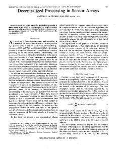
Figure 1: Circuit based on the ZPM for reading the array of resistive sensors. The position of the switches allows the reading of R12 .

R11

R12

R1N

R21

R22

R2N

RM1

RM2

RMN

I1 (1,2) Vc1

Vr1

Vr2

VrM

I2 (1,2) Vc2

IN (1,2) VcN

2. Reading an Array of Resistive Sensors Using ZPM and VFM Circuits The simplest circuit for reading an array of resistive sensors based on the ZPM is shown in Figure 1. The reading procedure for this circuit consists of selecting, using the row selection switches, a positive voltage for one of the wires of row i 1 ≤ i ≤ M , while the rest are connected to ground. Likewise, all column wires except one, j 1 ≤ j ≤ N , are connected to ground. Meanwhile, the column switch j connects the wire of the jth array column to the inverting input of the OA. Using this switch layout (if the switches were ideal), there is only current flowing through the sensor connected to row i and column j, since voltages Vri of the row wires and Vc j of the column wires of the array of Figure 1 would be V DD or ground, depending on the selection in the switches. This current could be calculated by the following expression: Rij = −

V DD Rf , Vo i, j

1

Io (1,2) Rg

+ − Vo

Figure 2: Circuit based on the VFM for reading the array of resistive sensors. The position of the switches allows the reading of R12 .

where Vo i, j is the output voltage of the OA when the switch of row i selects V DD and the switch of column j connects this column’s wire to the inverting input terminal of the OA. Unfortunately, (1) is merely an approximation to the real value of Rij , since voltages Vri and Vc j do not match V DD or ground due to the resistances of the switches, Rs. On the other hand, Figure 2 shows a circuit that uses the VFM for the array reading. This circuit is a slightly modified version of the classical VFM circuits that uses a single

Journal of Sensors

3

resistor, Rg (as shown in Figure 2), rather than the one with the same value for each of the columns of the array, such as in [16]. The readout procedure consists of using the row selection switches to select a positive voltage, V DD , for one of the row wires, i, while the rest are connected to the output of the OA. Moreover, all column switches except one, j, are connected to the output voltage of the OA. The column switch, j, connects the wire of this column to the resistor, Rg, which in turn is connected to the noninverting input terminal of the OA. Once again, if the row and column switches were ideal, only the current would flow through the resistor Rij , the value of which could be calculated by the following expression: Rij =

V DD − 1 ⋅ Rg, Vo i, j

R11

R12

R1N

R21

R22

R2N

RM1

RM2

RMN

2 + −

where Vo i, j is the output voltage of the OA when the switch of row i selects V DD and the switch of column j connects this column’s wire to the noninverting input terminal of the OA. As in the case of the ZPM circuit, (2) would only be valid if the resistors of the column and row switches, Rs, are 0. The error that occurs in estimating Rij using these equations will depend on Rs, on the size of the array (M and N), and the range of values of the resistances of the sensors [16, 26]. To reduce the errors due to Rs in (1), Wu et al. [31] propose modifying the circuit based on the ZPM of Figure 1 by adding a second OA and a resistor (Figure 3). For this circuit, Wu et al. propose calculating Rij , with the value of Rs known, according to the following equation: Rij = − V DD + Vcg ⋅

Rs Rl − 2Rs, Rcg VLij

V DD V DD − 1 ⋅ Rg + ⋅ Rs Vo i, j Vo i, j

VLij

Rcg

Vcg

Figure 3: Modified circuit based on the ZPM proposed by Wu et al. [31] to reduce the influence of Rs in calculating Rij .

R11

R12

R1N

R21

R22

R2N

RM1

RM2

RMN

3

Vcg and VLij are the output voltages of the OAs in Figure 3 and Rl and Rcg are the feedback resistors of these OAs (as one example in Figure 3, multiplexers are selected to the readout of R11 ). Although the circuit in Figure 3 reduces the number of parasitic parallel paths due to Rs, these are not completely eliminated and, therefore, expression (3) still shows errors in estimating Rij . These errors again depend on Rs, on the size of the array, and on the resistors to be measured. Based on the VFM, in [26], Wu et al. propose a new design (Figure 4) in order to reduce crosstalk. Wu et al. propose evaluating Rij according to the following equation: Rij =

+ −

Rl

4

The second term of the member on the right is the only difference from (2). Although, for some ranges of Rij and Rs, the errors using (4) for the circuit of Figure 4 are smaller than

Rg Rg

+ − Rs Vo

Figure 4: Modified circuit based on the VFM proposed by Wu et al. [26] to reduce the effects of crosstalk.

those obtained using (2) for the circuit (Figure 2), these errors do not disappear.

3. Method for Reducing Crosstalk Errors in Reading an Array of Resistive Sensors To reduce errors, due to the resistances of the switches that appear in (1), (2), (3), and (4), a new method to calculate Rij is presented in this section. The method is the

4

Journal of Sensors R11 IR (i) 1j

same, with minor modifications, for the simplest version of the ZPM- and VFM-based circuits (Figures 1 and 2). In essence, the method uses the estimates values of Rij by using (1) and (2) as the starting point to obtain the voltages in the row and column wires of the array (Vri and Vc j ) that will be used to, in successive steps, improve the estimation of Rij . The method is described below in its two variants.

Vr1 Ri1

R1j

IRij (i)

RMj

RM1 IRMj (i)

Vc1 (i) Rs

0

V DD Rf , Vo i, j

Rs

Rs

RMN

VrM Rs

Ij (i)

Vcj (i)

, through (1): Rij = −

RiN Vri

3.1. Method for Reducing Crosstalk Errors in Reading Circuits Based on ZPM. For the circuit of Figure 1, the proposed method begins by obtaining an initial estimation of all Rij ,

0 Rij

R1N

R1j

VcN (i)

Rs

Rs

Io (i,j)

5

+ − Rf

where the superscript will indicate the current step of the process. Next, if resistors of multiplexers, Rs, are considered for improving accuracy in the readout of Rij , it is necessary to analyse the equivalent circuit in Figure 5. In this circuit, the current flowing towards the Rf resistor when connecting the wire of row i to V DD and the wire of column j to the OA, Io i, j , is Io i, j = −

Vo i, j = Ij i , Rf

Figure 5: Equivalent circuit, based on the ZPM, including the resistor of multiplexers Rs for improving accuracy in the readout of Rij .

and replacing Vcp i from (7):

6

0

1

where I j i is the current flowing through the multiplexer of the jth column wire (see Figure 5). It should be noted that I j i does not depend on the column selected for reading since, in any selection state of the column switches, these connect the columns of the array at a voltage of 0 V. This current is used to calculate the voltage values of the column wires in Figure 5, Vc j i = I j i ⋅ Rs = −Vo i, j

Vo

Rs , Rf

Vrk i =

0

N

〠p=1 Y kp

+ Ys

0

,

9

0

Y kp and Ys are the inverse of Rkp and Rs, respectively, while δik is the Kronecker delta. On the other hand, the 1 current passing through Rij in this first step, IRij (see Figure 5), is

7

where Vc j i is the voltage of the wire of column j when connecting row i to V DD . The recursive process begins by calculating the voltages of any row wire in the array, k, when V DD is connected row 1 wire i: Vrk i (note that Vrk do not depend on which column is selected). This voltage can be calculated using Millman’s theorem [32] and (7) as

V DD ⋅ Ys ⋅ δik − Rs/Rf ⋅ 〠Np=1 Vo i, p Y kp

M

1

1

IRij = Io i, j − 〠 IRkj k=1,k≠i M

= Io i, j − 〠 k=1,k≠i

=−

Vo i, j Rf

1

0

Vrk i − Vc j i M

0

1 + Rs ⋅ 〠 Y kj k=1,k≠i

⋅ Y kj M

1

0

− 〠 Vrk i ⋅ Y kj k=1,k≠i

10

0

1

Vrk i =

V DD ⋅ Ys ⋅ δik + 〠Np=1 Vcp i ⋅ Y kp 0 N 〠p=1 Y kp

1 Rij

=

Vri

1

+ Ys

i − Vc j i IR1ij

=

8

1

Now, Rij can be found using the results of (5), (6), (7), (8), and (9):

Vri − Vo i, j /Rf

1

i + Vo i, j Rs/Rf 0

1 + Rs ⋅ 〠M k=1,k≠i Y kj

1

0

− 〠M k=1,k≠i Vrk i ⋅ Y kj

11

Journal of Sensors

5

i would be calculated using (9), with step (instead of q

q

0 Rij

q−1 Rij

R1j

R11 IR (i,j) 1j

Equations (9) and (11)are the recursive equations of the q proposed method. Thus, in the qth step, new values of Vrk

R1N

from the q − 1 Ri1

). The step finishes using (11) to calculate

Rij

IRij (i,j)

RiN

3.2. Method for Reducing Crosstalk Errors in Reading Circuits Based on VFM. For the circuit in Figure 2, the method is very similar to the one presented in the previous subsection, begin0 ning with the calculation of all the Rij from (2). Again, if Rs is considered, it is necessary to analyse the circuits of Figure 6 for improving accuracy. In this circuit, the current flowing towards the Rg resistor when switching row i to V DD and connecting column j to the OA, Io i, j , is calculated: Vo i, j Rg

RM1 IR

Mj

+ Ys V DD ⋅ δik + Vo i, j ⋅ 1 − δik N

0

Rs

Rs

+ −

Rg

Figure 6: Equivalent circuit, based on the VFM, including the resistor of multiplexers Rs for improving accuracy in the readout of Rij .

13

1

Vrk i, j = Vo i, j N

⋅

⋅ Ys

1+

+

0

Rs/Rg ⋅ 〠t=1 V DD − Vo i, j /V DD − Vo i, t N

⋅ Vo i, t /Vo i, j ⋅ Y kt

0

〠t=1 Y kt + Ys

V DD − Vo i, j ⋅ δik ⋅ Ys N

0

〠t=1 Y kt + Ys

16 The current passing through Rij when selected row i and 1

column j (in the first step of the recursive method) IRij i, j is (see Figure 6):

14

M

1

1

IRij i, j = Io i, j − 〠 IRkj i, j k=1,k≠i M

= Io i, j − 〠 k=1,k≠i

1

Vc j i, j − Vrk i, j

0

⋅ Y kj

M Vo i, j Rs 0 ⋅ 〠 Y kj = − Vo i, j ⋅ 1 + Rg Rg k=1,k≠i

0 ⋅ Y kt

〠t=1 Y kt

IN (i,j)

VcN (i)

Io (i,j)

The recursive process for this circuit starts by using Millman’s theorem and (14) to recalculate the voltages of kth row of the array when selecting for reading row i and column j, 1 Vr k i, j :

+

Rs

Vo

Vct i, j = I t i, j ⋅ Rs + Vo i, j Rs V DD − Vo i, j ⋅ = Vo i, t ⋅ + Vo i, j Rg V DD − Vo i, t

j

RMN

Ij (i,j)

Vcj (i)

Rs

This equation shows the effect of the voltage scaling that has taken place in the array when column t or column j was selected (keeping i as the selected row). Having in mind that I t i, t = Io i, t , (12) and (13) can be used to calculate the voltage in the wire of the column t when selecting row i and column j, Vct i, j :

1

I1 (i,j)

Vc1 (i)

12

I t i, j V − Vo i, j = DD I t i, t V DD − Vo i, t

Vrk i, j =

RMj

(i,j)

VrM

For this circuit (if any row i is selected), it is possible to find the current flowing through the switch of a selected column t, I t i, t as a function of the current flowing through the switch of the same column, when another column j was selected:

N 〠t=1 Vct i, 0 N 〠t=1 Y kt

Rs

Vri

1

Rij with Vrk i instead of Vrk i .

Io i, j =

Rs

Vr1

15

M

1

17

0

+ 〠 Vrk i, j ⋅ Y kj

+ Ys

k=1,k≠i

1

Thus, Rij can be calculated as

or

1

Rij =

Vri

1

i, j − Vc j i, j 1 IRij

i, j

=

Vri

1

i, j − Vo i, j ⋅ 1 + Rs/Rg 0

1

1

M Vo i, j /Rg − Vo i, j ⋅ 1 + Rs/Rg ⋅ 〠M k=1,k≠i Y kj + 〠k=1,k≠i Vrk i, j ⋅ Y kj

18

6

Journal of Sensors

Table 1: Comparison of the results obtained in an 8 × 8 array with different values of Rij if Rs = 1 Ω and the rest of the resistors of the array, Rns, take different values. (a) Classical approach. (b) ZPM circuit proposed by Wu et al. (c) Results for the proposed method in the first step. (d) Results for the proposed method in the second step. (a) ZPM classical approach Rs = 1 Ω Rns (Ω) 100 200 300 400 600 800 1200 1800 3000 6000 10000

100

500

16.00 9.10 6.73 5.55 4.36 3.77 3.18 2.79 2.47 2.24 2.14

12.39 7.19 5.02 3.88 2.73 2.15 1.57 1.18 0.87 0.63 0.54

Error (%), Rij (Ω) 2000 5000 7500 5.48 5.95 4.42 3.44 2.38 1.82 1.25 0.86 0.55 0.32 0.23

5.68 4.07 3.77 3.11 2.22 1.70 1.15 0.78 0.47 0.24 0.15

13.30 2.59 3.27 2.88 2.12 1.64 1.11 0.74 0.44 0.21 0.12

10000 19.78 1.16 2.79 2.65 2.03 1.58 1.08 0.72 0.42 0.19 0.10

100 200 300 400 600 800 1200 1800 3000 6000 10000

100

500

97.34 15.26 10.83 18.78 1.16 0.87 0.58 0.39 0.23 0.12 0.07

68.28 84.06 72.51 54.82 1.15 0.87 0.58 0.39 0.23 0.11 0.07

100

500

100 200 300 400 600 800 1200 1800 3000 6000 10000

1.83 0.60 0.32 0.21 0.12 0.08 0.06 0.04 0.03 0.02 0.02

1.22 0.45 0.22 0.13 0.06 0.04 0.02 0.01 0.00 0.00 0.00

97.00 98.21 96.37 92.46 0.99 0.78 0.53 0.35 0.20 0.09 0.04

7500

10000

98.00 98.80 97.55 94.85 0.90 0.73 0.50 0.33 0.19 0.07 0.03

98.50 99.10 98.15 96.08 0.81 0.68 0.48 0.32 0.17 0.06 0.01

Error (%), Rij (Ω) 2000 5000 7500 0.35 0.28 0.16 0.09 0.04 0.01 0.00 0.01 0.01 0.01 0.01

500

100 200 300 400 600 800 1200 1800 3000 6000 10000

0.24 0.04 0.02 0.01 0.00 0.00 0.00 0.00 0.00 0.00 0.00

0.14 0.02 0.00 0.00 0.00 0.00 0.00 0.00 0.00 0.00 0.00

Error (%), Rij (Ω) 2000 5000 7500 0.13 0.02 0.02 0.02 0.02 0.02 0.02 0.01 0.01 0.01 0.01

0.64 0.10 0.07 0.06 0.05 0.05 0.04 0.04 0.03 0.03 0.03

1.06 0.17 0.12 0.10 0.08 0.07 0.06 0.06 0.05 0.05 0.04

10000 1.48 0.23 0.16 0.13 0.11 0.09 0.08 0.07 0.07 0.06 0.06

For VFM-based circuits, (16) and (18) are the recursive equations of the proposed method. Thus, in the qth step, q new values of Vrk i, j would be calculated using (16), with q−1

Rij

0

founded in the q − 1 step (instead of Rij ). The step finq

q

Vrk i, j .

(c) ZPM proposed method, 1st step Rs = 1 Ω Rns (Ω)

100

1

Error (%), Rij (Ω) 2000 5000 92.43 95.65 91.38 83.04 1.09 0.84 0.56 0.37 0.22 0.11 0.06

Rs = 1 Ω Rns (Ω)

ishes using (18) to calculate Rij with Vrk i, j instead of

(b) ZPM-Wu Rs = 1 Ω Rns (Ω)

(d) ZPM proposed method, 2nd step

3.30 0.01 0.06 0.03 0.00 0.02 0.03 0.03 0.03 0.03 0.03

5.62 0.26 0.02 0.02 0.03 0.04 0.05 0.05 0.05 0.05 0.04

10000 7.84 0.50 0.10 0.06 0.06 0.07 0.07 0.07 0.06 0.06 0.06

4. Results and Discussion To compare the results provided by the proposed methods to those provided by the classical equations of the ZPM and VFM circuits, (1) and (2), and also the results of the circuits proposed by Wu et al., (3) and (4), a batch of simulations has been carried out using Cadence Orcad-Pspice 16.6. A general purpose OA, the Texas Instrument OPA4188, was used for the readout circuit in every test with the power supplies adjusted to +5 V and −5 V. The OA is designed with autozeroing techniques to provide low offset voltage (25 μV, maximum) and near zero-drift over time and temperature. The DC gain is 136 dB, and the input bias current is 16 pA. Errors due to the nonidealities of the OA are minimized thanks to these characteristics. If, for example, the offset voltage of the OA was higher, the technique reported in [22] could be used to reduce its influence. The sensing resistor Rij range used for simulation was [100 Ω, 10 kΩ]. This range is typically for touch sensors [33]. Another reason to use this range of resistors is that it shows the difference in operation and limitations of circuits based on the ZPM and VFM, as will be shown in the results. For this range of sensor resistors, Rf = 75 Ω, Rg = 350 Ω, Rl = 75 Ω, and Rcg = 75 Ω have been selected in order not to saturate the output voltages of the OA and to ensure the difference between the maximum and the minimum Vo which is approximately equal in all circuits. In general, simulations will be presented to compare the operation of the circuits of Figures 1 and 2 (evaluated, resp., by (1) and (2) and hereinafter classical approach), the two circuits of Figures 3 and 4 proposed by Wu et al. (evaluated, resp., by (3) and (4) and hereinafter ZPM-Wu and VFM-Wu), and the proposed method presented in the previous section.

Journal of Sensors

7

Table 2: Comparison of the results obtained in an 8 × 8 array with different values of Rij if Rns = 5 kΩ and the resistances of the switches take different values. (a) Classical approach. (b) ZPM circuit proposed by Wu e al. (c) Results for the proposed method in the first step. (d) Results for the proposed method in the second step. (a) ZPM classical approach Rns = 5 kΩ Rs (Ω) 1 2 4 6 9 15 20 25

100

500

2.28 4.57 9.17 13.79 20.76 34.86 46.77 58.82

0.68 1.36 2.73 4.10 6.17 10.35 13.87 17.42

Error (%), Rij (Ω) 2000 5000 7500 0.37 0.75 1.51 2.27 3.42 5.73 7.67 9.61

0.29 0.61 1.25 1.89 2.85 4.77 6.36 7.96

0.26 0.57 1.18 1.79 2.70 4.52 6.03 7.54

10000 0.24 0.54 1.13 1.73 2.62 4.38 5.84 7.29

(b) ZPM-Wu Rns = 5 kΩ Rs (Ω)

100

500

1 2 4 6 9 15 20 25

0.14 0.28 0.56 0.84 1.26 2.09 2.79 3.48

0.14 0.28 0.56 0.84 1.25 2.09 2.78 3.47

Error (%), Rij (Ω) 2000 5000 7500 0.13 0.27 0.55 0.82 1.24 2.06 2.75 3.42

0.11 0.25 0.53 0.80 1.21 2.02 2.68 3.33

0.10 0.24 0.51 0.78 1.19 1.98 2.63 3.26

10000 0.08 0.22 0.49 0.77 1.17 1.95 2.57 3.18

(c) ZPM proposed method, 1st step Rns = 5 kΩ Rs (Ω)

100

500

1 2 4 6 9 15 20 25

0.03 0.10 0.38 0.80 1.67 4.07 6.56 9.39

0.00 0.01 0.04 0.09 0.20 0.55 0.94 1.43

Error (%), Rij (Ω) 2000 5000 7500 0.01 0.01 0.01 0.03 0.08 0.23 0.41 0.63

0.03 0.03 0.02 0.00 0.04 0.16 0.31 0.48

0.05 0.04 0.03 0.02 0.02 0.14 0.27 0.44

10000 0.06 0.06 0.05 0.03 0.00 0.11 0.24 0.40

(d) ZPM proposed method, 2nd step Rns = 5 kΩ Rs (Ω)

100

500

1 2 4 6 9

0.00 0.00 0.02 0.06 0.17

0.00 0.00 0.00 0.00 0.00

Error (%), Rij (Ω) 2000 5000 7500 0.01 0.01 0.01 0.01 0.01

0.03 0.03 0.03 0.03 0.03

0.05 0.05 0.05 0.05 0.05

10000 0.06 0.06 0.06 0.06 0.06

Table 2: Continued. Rns = 5 kΩ Rs (Ω)

100

500

15 20 25

0.63 1.26 2.12

0.03 0.07 0.14

Error (%), Rij (Ω) 2000 5000 7500 0.00 0.01 0.03

0.03 0.02 0.00

0.04 0.03 0.02

10000 0.06 0.05 0.04

Table 1 shows simulation results for the different circuits and methods presented based on the ZPM. The aim of this series of simulations is to analyse the influence of nonscanned resistors, Rns, on the measurement of the resistor, Rij . In all cases, it is an 8 × 8 array in which the resistance of the switches is set to 1 Ω (a resistance that is relatively easy to obtain for switches). Different values of Rns are used for each value of the resistor to be measured, Rij . Both Rns and Rij vary in the selected range [100 Ω, 10 kΩ]. In the first place, it should be noted that the errors for Rns < 600 Ω are very large in the case of the ZPM-Wu circuit, Table 1(b). This is due to the additional OA decreasing its output voltage as the current flowing through the parasitic parallel paths increases (which occurs for low values of Rns), reaching a point at which its output becomes saturated. On the other hand, the four tables of Table 1 show how the errors are greater as Rns decreases. This is justified again by the increase in the current in the parasitic parallel paths with lower values of Rns. With the exception of cases in which Rns is low, the errors in the ZPM-Wu circuit are always lower than those that appear in the ZPM evaluated using the classical approach (Table 1(a)). For its part, the proposed method outperforms the previous methods. It can be seen how the convergence of this method is very fast, since better results are obtained in the first step (Table 1(c)) than with the other two methods (except for errors below 0.03% in ZPM-Wu). In the second step, the maximum error obtained is only 1.48%, more than an order of magnitude lower than that obtained by the classical approach, and with better results in all situations. It also improves the results of the ZPM-Wu circuit in all situations for errors over 0.06%. The results provided in Table 1(a) quite closely match those reported in [10] for a 10 × 10 array, in which the aim is to measure the value of a sensor when the rest of the sensors has resistances between 3 kΩ and 19 kΩ. The aim of the simulations presented in Table 2 is to analyse the influence of the resistances of the switches, Rs, on the reading of Rij . In the first place, it is observed how the errors increase for the classical approach and for ZPM-Wu when Rs is increased. The same happens when the value of Rij decreases. The proposed method also shows these trends, except when the errors are very low (below 0.06%). For any combination of Rns and Rs, the results obtained by the proposed method in the second step outperform the results of the other methods. Even in the first step, except for Rij = 100 Ω and Rs > 9 Ω, the results are better than in the other methods. It should be noted that the maximum error in the second step is only 2.12% when the resistances of the switches are a quarter of the value to be measured.

8

Journal of Sensors

Table 3: Results obtained for methods based on the VFM in an 8 × 8 array with different values of Rij if Rs = 1 Ω and the rest of the resistors in the array, Rns, take different values. (a) Classical approach. (b) VFM circuit proposed by Wu et al. (c) Results for the proposed method in the first step. (d) Results for the proposed method in the second step. (a) VFM classical approach Rs = 1 Ω Rns (Ω) 100 200 300 400 600 800 1200 1800 3000 6000 10000

100

500

13.85 9.17 6.79 5.60 4.40 3.81 3.21 2.81 2.50 2.26 2.16

80.64 54.87 14.46 3.92 2.76 2.18 1.59 1.19 0.88 0.64 0.55

Error (%), Rij (Ω) 2000 5000

7500

10000

98.67 96.75 93.42 86.12 2.24 1.75 1.21 0.83 0.52 0.28 0.18

99.00 97.56 95.05 89.53 2.18 1.72 1.20 0.82 0.51 0.28 0.18

Error (%), Rij (Ω) 2000 5000 7500

10000

93.09 83.35 66.77 31.97 0.27 0.24 0.22 0.22 0.22 0.22 0.22

98.61 96.61 93.13 85.45 0.47 0.33 0.27 0.25 0.25 0.25 0.25

95.03 88.01 76.08 51.04 2.43 1.86 1.28 0.89 0.58 0.34 0.25

98.00 95.14 90.19 79.41 2.30 1.78 1.22 0.84 0.52 0.29 0.19

(b) VFM-Wu Rs = 1 Ω Rns (Ω)

100

500

100 200 300 400 600 800 1200 1800 3000 6000 10000

0.19 0.54 0.66 0.69 0.72 0.72 0.73 0.73 0.74 0.74 0.74

73.03 37.21 0.19 0.12 0.09 0.08 0.07 0.07 0.07 0.07 0.07

97.22 93.25 86.38 71.40 0.36 0.29 0.26 0.25 0.25 0.25 0.25

98.14 95.49 90.87 80.71 0.41 0.31 0.26 0.25 0.25 0.25 0.25

(c) VFM proposed method, 1st step Rs = 1 Ω Rns (Ω) 100 200 300 400 600 800 1200 1800 3000 6000 10000

100

500

27.48 0.31 0.04 0.03 0.12 0.12 0.08 0.07 0.05 0.05 0.04

83.53 58.05 18.45 0.17 0.09 0.06 0.04 0.02 0.02 0.01 0.01

Error (%), Rij (Ω) 2000 5000 95.76 88.85 77.19 52.71 0.05 0.05 0.04 0.03 0.02 0.01 0.01

98.30 95.48 90.64 80.11 0.02 0.06 0.04 0.03 0.02 0.02 0.01

7500

10000

98.86 96.98 93.72 86.59 0.07 0.08 0.05 0.03 0.03 0.02 0.02

99.15 97.73 95.28 89.88 0.08 0.02 0.05 0.04 0.03 0.02 0.02

(d) VFM proposed method, 2nd step Rs = 1 Ω Rns (Ω) 100 200 300 400 600 800 1200 1800 3000 6000 10000

100

500

29.45 1.00 0.38 0.19 0.00 0.04 0.03 0.03 0.02 0.02 0.02

83.93 58.27 18.63 0.04 0.03 0.02 0.02 0.01 0.01 0.01 0.01

Error (%), Rij (Ω) 2000 5000 95.87 88.91 77.24 52.77 0.03 0.01 0.02 0.02 0.01 0.01 0.01

98.34 95.50 90.66 80.14 0.03 0.03 0.02 0.01 0.01 0.01 0.01

7500

10000

98.89 96.99 93.74 86.60 0.04 0.04 0.03 0.03 0.02 0.02 0.02

99.17 97.74 95.29 89.89 0.04 0.04 0.04 0.03 0.03 0.02 0.02

Table 3 shows simulation results for the different circuits and methods presented based on the VFM. The aim of this series of simulations is to analyse the influence of nonscanned resistors, Rns, on the measurement of the resistor, Rij . Again, it is an 8 × 8 array in which the resistance of the switches is set to 1 Ω. Different values of Rns are used for each value of the resistor to be measured, Rij . Both Rns and Rij vary in the selected range [100 Ω, 10 kΩ]. The first question to consider is that the errors for any method are very large if Rns < 600 Ω. This comes about since the parasitic current flowing through the Rns of row i is excessive for the OA (even though the feedback resistor, Rg, has been chosen so there is no saturation of voltages of the OA in the selected range of individual resistors). The situation gets worse with increased Rij , since Vo i, j decreases, and in consequence, the current flowing through all the Rns of row i increases. This situation does not occur in the ZPM circuits since the row selection switches are responsible for providing this current. The range limitation of Rns is therefore a drawback of VFM-based circuits compared to those based on the ZPM. It is worth to note that situations with all Rns very low are uncommon in arrays of sensors. For example, in [33], a 16 × 16 tactile sensor array designed with a continuous electroactive material using a piezoresistive sheet of capLINQ (code MVCF40012BT50KS/2A) has 10 kΩ for no-pressed tactels; however, only the few pressed ones might have resistances around 300 Ω. If this saturation does not come about (due to the current to be provided by the OA), the proposed method outperforms the other methods in both the first and the second steps for all combinations of Rij and Rns. Finally, the results obtained by the proposed method are very similar in the VFM and ZPM circuits (outside of the saturation range of the VFM circuit). Table 4 shows the influence of the resistances of the switches, Rs, on the error in estimating Rij for the methods based on the VFM. Once again, the error increases with the value of Rs and, except for VFM-Wu, also increases with decreasing Rij . The biggest errors occur, as in all previous cases, for the classical approach, while the proposed method

Journal of Sensors

9

Table 4: Results obtained for methods based on the VFM in an 8 × 8 array with different values of Rij if Rns = 5 kΩ and the resistances of the switches take different values. (a) Classical approach. (b) VFM circuit proposed by Wu et al. (c) Results for the proposed method in the first step. (d) Results for the proposed method in the second step. (a) VFM classical approach Rns = 5 kΩ Rs (Ω) 1 2 4 6 9 15 20 25

100

500

2.31 4.59 9.19 13.81 20.78 34.88 46.79 58.85

0.69 1.37 2.74 4.12 6.19 10.36 13.88 17.43

Error (%), Rij (Ω) 2000 5000 7500 0.39 0.77 1.53 2.30 3.45 5.76 7.69 9.64

0.34 0.66 1.30 1.94 2.90 4.82 6.42 8.02

0.33 0.63 1.24 1.86 2.77 4.59 6.11 7.62

10000 0.32 0.62 1.22 1.82 2.71 4.48 5.94 7.39

(b) VFM-Wu Rns = 5 kΩ Rs (Ω) 1 2 4 6 9 15 20 25

100

500

0.74 0.16 0.98 2.12 3.83 7.23 10.05 12.86

0.07 0.64 1.76 2.85 4.47 7.58 10.07 12.46

Error (%), Rij (Ω) 2000 5000 7500 0.22 0.79 1.90 2.99 4.59 7.66 10.09 12.41

0.25 0.81 1.93 3.02 4.62 7.69 10.12 12.45

0.25 0.82 1.93 3.02 4.63 7.71 10.15 12.49

10000 0.25 0.82 1.93 3.03 4.63 7.72 10.18 12.54

(c) VFM proposed method, 1st step Rns = 5 kΩ Rs (Ω)

100

500

1 2 4 6 9 15 20 25

0.05 0.12 0.40 0.82 1.70 4.09 6.59 9.42

0.01 0.02 0.05 0.11 0.22 0.56 0.96 1.45

Error (%), Rij (Ω) 2000 5000 7500 0.01 0.01 0.03 0.05 0.10 0.25 0.44 0.65

0.02 0.02 0.03 0.05 0.09 0.21 0.36 0.54

0.02 0.02 0.03 0.05 0.09 0.21 0.34 0.51

10000 0.02 0.03 0.04 0.05 0.09 0.21 0.34 0.50

(d) VFM proposed method, 2nd step Rns = 5 kΩ Rs (Ω)

100

500

1 2 4 6 9

0.02 0.02 0.04 0.08 0.19

0.01 0.01 0.01 0.01 0.02

Error (%), Rij (Ω) 2000 5000 7500 0.01 0.01 0.01 0.01 0.01

0.02 0.02 0.02 0.02 0.02

0.02 0.02 0.02 0.02 0.02

10000 0.02 0.02 0.02 0.02 0.03

Table 4: Continued. Rns = 5 kΩ Rs (Ω)

100

500

15 20 25

0.66 1.29 2.15

0.05 0.09 0.16

Error (%), Rij (Ω) 2000 5000 7500 0.03 0.04 0.06

0.02 0.04 0.05

0.03 0.04 0.05

10000 0.03 0.04 0.06

presents the best results for all combinations, even in the first step. Comparing the errors obtained for ZPM-based methods to the errors of VFM-based methods, it is found that they are quite similar for the classical approach. The errors are similar (although slightly higher) in both steps for the proposed methods and a great deal higher in the case of VFM-Wu. Two sets of simulations have been carried out for the circuits of the ZPM of Table 5 and the VFM of Table 6 in order to analyse the errors by changing the size of the array. In both simulations, Rs = 5 Ω and Rns = 2 kΩ. For all methods, errors increase for bigger arrays. The classical approach shows higher errors than Wu proposals, while the proposed methods give the lowest errors. On the other hand, very similar errors appear for the classical approach in both circuits while errors in ZPM-Wu are lower than those obtained in VFM-Wu. It is worth noting that the proposed method shows the best results in all cases and, when the size increases, the advantage grows. So when the size varies from 4 × 4 to 16 × 16, errors for the proposed methods in the biggest array are less than the error for the smallest array with the other approaches.

5. Conclusions The main problem in determining sensor resistances in a resistive array is the appearance of crosstalk. This phenomenon is due mainly to the resistance of the sensor selection switches to be measured. Crosstalk appears in the two types of circuits known in the literature for reading the array: the zero potential method (ZPM) and the voltage feedback method (VFM). This article presents a recursive method to obtain the individual values of the resistors in an array of resistive sensors that reduces the influence of crosstalk in determining the resistances of the sensors. The new method proposed is similar for both types of circuits and is based on the recursive calculation of the row and column voltages of the array. The proposed method converges very quickly, outperforming, in its first or second iteration, the classical equations of the ZPM and VFM and also the circuits proposed by Wu to reduce errors. The method does not require any additional hardware and is applied directly to the classic ZPM and VFM circuits. The errors found in the calculations using the proposed method are similar for both types of circuit and increase slowly as the array size and selection switch resistance increase. As a further conclusion, it should be noted that a decrease has been observed in the range of resistance values that can be measured in VFM circuits compared to ZPM circuits for equal output voltage ranges.

10

Journal of Sensors

Table 5: Results obtained for methods based on the ZPM by changing the size of the array and maintaining Rns = 2 kΩ and Rs = 5 Ω. (a) Classical approach. (b) ZPM circuit proposed by Wu et al. (c) Results for the proposed method in the first step. (d) Results for the proposed method in the second step. (a) ZPM classical approach Rns = 2 kΩ Size 4×4 6×6 8×8 10 × 10 12 × 12 14 × 14 16 × 16

100

500

11.58 12.63 13.69 14.76 15.83 16.91 17.99

3.51 4.53 5.55 6.57 7.59 8.62 9.66

Error (%), Rij (Ω) 2000 5000 7500 1.99 2.99 3.98 4.98 5.98 6.98 7.98

1.66 2.64 3.61 4.58 5.54 6.49 7.43

1.57 2.53 3.49 4.43 5.35 6.26 7.16

10000 1.51 2.46 3.39 4.31 5.20 6.07 6.93

Table 6: Results obtained for methods based on the VFM by changing the size of the array and maintaining Rns = 2 kΩ and Rs = 5 Ω. (a) Classical approach. (b) VFM circuit proposed by Wu et al. (c) Results for the proposed method in the first step. (d) Results for the proposed method in the second step. (a) VFM classical approach Rns = 2 kΩ Size 4×4 6×6 8×8 10 × 10 12 × 12 14 × 14 16 × 16

100

500

11.60 12.66 13.72 14.79 15.86 16.94 18.02

3.53 4.54 5.56 6.59 7.62 8.65 9.68

(b) ZPM-Wu Rns = 2 kΩ Size

100

500

4×4 6×6 8×8 10 × 10 12 × 12 14 × 14 16 × 16

0.75 1.25 1.74 2.24 2.74 3.24 3.73

0.74 1.24 1.74 2.23 2.72 3.21 3.70

0.70 1.18 1.64 2.09 2.52 2.95 3.36

0.68 1.14 1.58 2.01 2.41 2.80 3.17

10000 0.66 1.11 1.53 1.93 2.30 2.65 2.98

Rns = 2 kΩ Size 4×4 6×6 8×8 10 × 10 12 × 12 14 × 14 16 × 16

(c) ZPM proposed method, 1st step Rns = 2 kΩ Size

100

500

4×4 6×6 8×8 10 × 10 12 × 12 14 × 14 16 × 16

0.58 0.70 0.84 0.99 1.15 1.33 1.52

0.07 0.13 0.20 0.29 0.40 0.52 0.66

0.00 0.03 0.09 0.16 0.24 0.33 0.44

0.02 0.01 0.06 0.13 0.21 0.29 0.39

10000

100

500

4×4 6×6 8×8 10 × 10 12 × 12 14 × 14 16 × 16

0.03 0.05 0.06 0.08 0.10 0.13 0.16

0.00 0.00 0.00 0.01 0.02 0.03 0.04

Error (%), Rij (Ω) 2000 5000 7500 0.01 0.01 0.01 0.01 0.00 0.01 0.02

0.03 0.03 0.03 0.03 0.03 0.02 0.01

100

500

10.77 11.27 11.77 12.27 12.77 13.27 13.77

2.76 3.26 3.75 4.25 4.74 5.24 5.73

0.04 0.01 0.04 0.10 0.17 0.25 0.34

Rns = 2 kΩ Size

100

500

4×4 6×6 8×8 10 × 10 12 × 12 14 × 14 16 × 16

0.61 0.73 0.87 1.02 1.18 1.15 0.07

0.08 0.14 0.22 0.31 0.42 0.55 0.68

(d) ZPM proposed method, 2nd step Rns = 2 kΩ Size

1.71 2.69 3.67 4.64 5.61 6.56 7.51

1.64 2.61 3.57 4.52 5.45 6.37 7.27

10000 1.60 2.56 3.50 4.43 5.33 6.21 7.07

Error (%), Rij (Ω) 2000 5000 7500 1.25 1.75 2.23 2.71 3.19 3.66 4.13

0.95 1.43 1.89 2.35 2.79 3.22 3.63

0.88 1.35 1.79 2.22 2.63 3.03 3.41

10000 0.84 1.30 1.73 2.13 2.52 2.88 3.21

(c) VFM proposed method, 1st step

Error (%), Rij (Ω) 2000 5000 7500 0.02 0.06 0.12 0.20 0.29 0.40 0.52

2.01 3.01 4.02 5.02 6.02 7.02 8.02

(b) VFM-Wu

Error (%), Rij (Ω) 2000 5000 7500 0.73 1.22 1.70 2.18 2.65 3.12 3.59

Error (%), Rij (Ω) 2000 5000 7500

0.05 0.05 0.05 0.05 0.05 0.05 0.04

Error (%), Rij (Ω) 2000 5000 7500 0.05 0.09 0.15 0.24 0.33 0.44 0.56

0.04 0.09 0.15 0.22 0.31 0.41 0.52

0.05 0.09 0.15 0.22 0.30 0.39 0.50

10000 0.05 0.09 0.15 0.22 0.30 0.38 0.48

(d) VFM proposed method, 2nd step

10000 0.06 0.07 0.07 0.07 0.07 0.07 0.06

Rns = 2 kΩ Size

100

500

4×4 6×6 8×8 10 × 10 12 × 12 14 × 14 16 × 16

0.06 0.07 0.09 0.11 0.13 0.08 1.56

0.01 0.02 0.02 0.03 0.04 0.06 0.07

Error (%), Rij (Ω) 2000 5000 7500 0.01 0.01 0.02 0.03 0.04 0.05 0.06

0.02 0.02 0.03 0.03 0.04 0.05 0.06

0.02 0.03 0.03 0.04 0.05 0.06 0.07

10000 0.02 0.03 0.04 0.04 0.05 0.06 0.07

Journal of Sensors

Data Availability The data used to support the findings of this study are available from the corresponding author upon request.

Conflicts of Interest The authors declare that they have no conflicts of interest.

References [1] I. Fratoddi, I. Venditti, C. Cametti, and M. V. Russo, “Chemiresistive polyaniline-based gas sensors: a mini review,” Sensors and Actuators B: Chemical, vol. 220, pp. 534–548, 2015. [2] J. Wang, S. Chan, R. R. Carlson et al., “Electrochemically fabricated polyaniline nanoframework electrode junctions that function as resistive sensors,” Nano Letters, vol. 4, no. 9, pp. 1693–1697, 2004. [3] A. Depari, M. Falasconi, A. Flammini et al., “A new low-cost electronic system to manage resistive sensors for gas detection,” IEEE Sensors Journal, vol. 7, no. 7, pp. 1073–1077, 2007. [4] D. Stratos, G. Maria, F. Eleftherios, and L. George, “Comparison of three resistor network division circuits for the readout of 4×4 pixel SiPM arrays,” Nuclear Instruments and Methods in Physics Research Section A: Accelerators, Spectrometers, Detectors and Associated Equipment, vol. 702, pp. 121–125, 2013. [5] J. F. Wu, L. Wang, J. Q. Li, and Z. Z. Yu, “A small size device using temperature sensor array,” Chinese Journal of Sensors and Actuators, vol. 24, pp. 1649–1652, 2011. [6] Y.-J. Yang, M.-Y. Cheng, S.-C. Shih et al., “A 32 × 32 temperature and tactile sensing array using PI-copper films,” The International Journal of Advanced Manufacturing Technology, vol. 46, no. 9-12, pp. 945–956, 2010. [7] M. Arlit, E. Schleicher, and U. Hampel, “Thermal anemometry grid sensor,” Sensors, vol. 17, no. 7, p. 1663, 2017. [8] W. Z. Wan Hasan, F. R. M. Rashidi, M. N. Hamidon, and Y. Wahab, “Design of readout circuit for piezoresistive pressure sensor using nodal array approach reading technique,” Pertanika Journal of Science & Technology, vol. 25, pp. 215–224, 2017. [9] W. E. Snyder and J. St. Clair, “Conductive elastomers as sensor for industrial parts handling equipment,” IEEE Transactions on Instrumentation and Measurement, vol. 27, no. 1, pp. 94–99, 1978. [10] L. Shu, X. Tao, and D. D. Feng, “A new approach for readout of resistive sensor arrays for wearable electronic applications,” IEEE Sensors Journal, vol. 15, no. 1, pp. 442–452, 2015. [11] F. Vidal-Verdú, M. J. Barquero, J. Castellanos-Ramos et al., “A large area tactile sensor patch based on commercial force sensors,” Sensors, vol. 11, no. 5, pp. 5489–5507, 2011. [12] Y. Wang, A. X. Wang, Y. Wang, M. K. Chyu, and Q.-M. Wang, “Fabrication and characterization of carbon nanotube–polyimide composite based high temperature flexible thin film piezoresistive strain sensor,” Sensors and Actuators A: Physical, vol. 199, pp. 265–271, 2013. [13] O. Oballe-Peinado, J. A. Hidalgo-Lopez, J. Castellanos-Ramos et al., “FPGA-based tactile sensor suite electronics for realtime embedded processing,” IEEE Transactions on Industrial Electronics, vol. 64, no. 12, pp. 9657–9665, 2017.

11 [14] M.-S. Suen, Y.-C. Lin, and R. Chen, “A flexible multifunctional tactile sensor using interlocked zinc oxide nanorod arrays for artificial electronic skin,” Sensors and Actuators A: Physical, vol. 269, pp. 574–584, 2018. [15] R. S. Saxena, N. K. Saini, and R. K. Bhan, “Analysis of crosstalk in networked arrays of resistive sensors,” IEEE Sensors Journal, vol. 11, no. 4, pp. 920–924, 2011. [16] H. Liu, Y.-F. Zhang, Y.-W. Liu, and M.-H. Jin, “Measurement errors in the scanning of resistive sensor arrays,” Sensors and Actuators A: Physical, vol. 163, no. 1, pp. 198–204, 2010. [17] T. D'Alessio, “Measurement errors in the scanning of piezoresistive sensors arrays,” Sensors and Actuators A: Physical, vol. 72, no. 1, pp. 71–76, 1999. [18] J. Wu, L. Wang, and J. Li, “VF-NSE method measurement error analysis of networked resistive sensor array,” Sensors and Actuators A: Physical, vol. 211, pp. 45–50, 2014. [19] J. A. Hidalgo-López, J. Romero-Sánchez, and R. FernándezRamos, “New approaches for increasing accuracy in readout of resistive sensor arrays,” IEEE Sensors Journal, vol. 17, no. 7, pp. 2154–2164, 2017. [20] Ó. Oballe-Peinado, F. Vidal-Verdú, J. Sánchez-Durán, J. Castellanos-Ramos, and J. Hidalgo-López, “Improved circuits with capacitive feedback for readout resistive sensor arrays,” Sensors, vol. 16, no. 2, p. 149, 2016. [21] J. S. Kim, D. Y. Kwon, and B. D. Choi, “High-accuracy, compact scanning method and circuit for resistive sensor arrays,” Sensors, vol. 16, no. 2, p. 155, 2016. [22] R. Yarahmadi, A. Safarpour, and R. Lotfi, “An improvedaccuracy approach for readout of large-array resistive sensors,” IEEE Sensors Journal, vol. 16, no. 1, pp. 210–215, 2016. [23] F. Reverter, F. Vidal-Verdú, and J. A. Hidalgo-Lopez, “Advanced techniques for directly interfacing resistive sensors to digital systems,” in Advanced Interfacing Techniques for Sensors: Measurement Circuits and Systems for Intelligent Sensors, B. George, J. K. Roy, V. J. Kumar, and S. C. Mukhopadhyay, Eds., pp. 139–165, Springer International Publishing, Cham, Switzerland, 2017. [24] J. F. Wu, “Scanning approaches of 2-D resistive sensor arrays: a review,” IEEE Sensors Journal, vol. 17, no. 4, pp. 914–925, 2017. [25] L. Wang, X.-L. Wen, J.-J. Pan, and L. Yang, “Improved FRZPC for the two-dimensional resistive sensor array,” IET Science, Measurement and Technology, vol. 12, no. 2, pp. 278–282, 2018. [26] J. Wu, L. Wang, and J. Li, “Design and crosstalk error analysis of the circuit for the 2-D networked resistive sensor array,” IEEE Sensors Journal, vol. 15, no. 2, pp. 1020–1026, 2015. [27] X. Zhang and X. Ye, “Zero potential method measurement error analysis for networked resistive sensor arrays,” IET Science, Measurement and Technology, vol. 11, no. 3, pp. 235–240, 2017. [28] J. Wu, L. Wang, J. Li, and A. Song, “A novel crosstalk suppression method of the 2-D networked resistive sensor array,” Sensors, vol. 14, no. 7, pp. 12816–12827, 2014. [29] J.-F. Wu, J.-Q. Li, and A.-G. Song, “Readout circuit based on double voltage feedback loops in the two-dimensional resistive sensor array: design, modelling and simulation evaluation,” IET Science, Measurement and Technology, vol. 11, no. 3, pp. 288–296, 2017. [30] F. Castro, T. Pentiado, J. Blanco, R. Xavier, M. Sanches, and A. de Carvalho, “Crosstalk error analysis in IIDFC readout

12 circuit for use in piezoresistive composite,” IEEE Sensors Journal, vol. 18, no. 1, pp. 382–389, 2018. [31] J.-F. Wu, F. Wang, Q. Wang, J.-Q. Li, and A.-G. Song, “An improved zero potential circuit for readout of a two-dimensional resistive sensor array,” Sensors, vol. 16, no. 12, p. 2070, 2016. [32] J. Millman, “A useful network theorem,” Proceedings of the IRE, vol. 28, no. 9, pp. 413–417, 1940. [33] J. A. Hidalgo-López, Ó. Oballe-Peinado, J. Castellanos-Ramos, J. A. Sánchez-Durán, R. Fernández-Ramos, and F. Vidal-Verdú, “High-accuracy readout electronics for piezoresistive tactile sensors,” Sensors, vol. 17, no. 11, 2017.

Journal of Sensors

International Journal of

Advances in

Rotating Machinery

Engineering Journal of

Hindawi www.hindawi.com

Volume 2018

The Scientific World Journal Hindawi Publishing Corporation http://www.hindawi.com www.hindawi.com

Volume 2018 2013

Multimedia

Journal of

Sensors Hindawi www.hindawi.com

Volume 2018

Hindawi www.hindawi.com

Volume 2018

Hindawi www.hindawi.com

Volume 2018

Journal of

Control Science and Engineering

Advances in

Civil Engineering Hindawi www.hindawi.com

Hindawi www.hindawi.com

Volume 2018

Volume 2018

Submit your manuscripts at www.hindawi.com Journal of

Journal of

Electrical and Computer Engineering

Robotics Hindawi www.hindawi.com

Hindawi www.hindawi.com

Volume 2018

Volume 2018

VLSI Design Advances in OptoElectronics International Journal of

Navigation and Observation Hindawi www.hindawi.com

Volume 2018

Hindawi www.hindawi.com

Hindawi www.hindawi.com

Chemical Engineering Hindawi www.hindawi.com

Volume 2018

Volume 2018

Active and Passive Electronic Components

Antennas and Propagation Hindawi www.hindawi.com

Aerospace Engineering

Hindawi www.hindawi.com

Volume 2018

Hindawi www.hindawi.com

Volume 2018

Volume 2018

International Journal of

International Journal of

International Journal of

Modelling & Simulation in Engineering

Volume 2018

Hindawi www.hindawi.com

Volume 2018

Shock and Vibration Hindawi www.hindawi.com

Volume 2018

Advances in

Acoustics and Vibration Hindawi www.hindawi.com

Volume 2018