Improving Measurement Accuracy in Sensor Networks by an Object Model Generation and Application. Leonid Reznik and Kurt Alfred Kluever. Department of ...
Improving Measurement Accuracy in Sensor Networks by an Object Model Generation and Application Leonid Reznik and Kurt Alfred Kluever Department of Computer Science Rochester Institute of Technology Rochester, New York, USA
Abstract— The paper describes a novel method of calculating measurement results in sensor networks, which includes modifying the conventional measurement estimates based on the object under measurement model mined from the data collected by the sensor network itself previously and other information made available by domain experts. It is shown that the model application might produce a significant gain in measurement accuracy if the model is correct. The gain value is estimated and its dependence on various factors is studied by computer simulation and experimentation with real sensor networks built from Crossbow Telos ver. B motes. The conditions of achieving the gain versus suffering the loss are derived and the recommendations of how to shape the object model in order to achieve and maximize the gain value are provided.
I.
INTRODUCTION
A model of an object or a process under measurement, which is called a measurement model in this paper, is traditionally used in many measurement procedures in order to improve the measurement result’s accuracy and reliability. A measurement model is developed as a dynamic multi-step transformation, usually conducted in a loop. The validity of the measurement model can be updated or modified as historical data are mined and processed. A novel technology of sensor networks has significantly enhanced our ability to collect more data to represent the object and environment under measurement, which allows for the development of more complex and complicated measurement models. Information necessary to develop a measurement model may come from two different sources: historical measurement results obtained by the same or similar sensor system and expert knowledge. Historical data need to be mined and processed in order to make them available for the model formulation. Both statistical methods and intelligent computational methodologies such as fuzzy logic, interval analysis, neural networks or genetic algorithms have been applied in data mining procedures. In addition to the historical data, domain experts can incorporate previous experience and general domain knowledge into the model.
Finally, the designers of the system being measured may provide knowledge of the design or operational characteristics of the sensors, network, etc. All of these factors are then folded into the final measurement model. This model could be written in a form of functional or other relationships, and may be approximate, stochastic or fuzzy. This paper attempts to apply the additional measurement model information, which is made in a form of predictions, for improving the accuracy of measurement results. The measurement model is formulated as a prediction model, which is often fuzzy due to the nature of the knowledge. We present the method that allows fusing various models with the data obtained from measurements in multi-channel sensor networks. It considers the stochastic models of the measurement results distribution (uniform distribution and normal distribution) along with fuzzy and interval models of the expert information. II.
INVESTIGATION OF
THE MODIFIED ESTIMATES VERSUS THE CONVENTIONAL ONES
We will compare the modified estimates of the measurements received with the application of fuzzy measurement models and the conventional estimates, which do not take the predictions into account. We will consider both interval and approximate value prediction models, in combinations with two of the most popular measurement results distributions: uniform distribution and normal distribution. This yields the following cases: A) uniform measurements distribution and interval prediction, B) normal measurements distribution and interval prediction, C) uniform measurements distribution and approximate value prediction, D) normal measurements distribution and approximate value prediction. Let us consider a prediction model information as a fuzzy constraint for the parameter vector X and given by the set of membership functions μi(fi(X)), i = 1,m, where m is the
number of predictions made by the experts. Each membership function describes one prediction model, typically about the possible value of the measurement result or a linear combination (for example, an average or a weighted average) of the measurement results. In this paper we will consider two functions commonly applied by experts: an interval prediction, where an expert’s prediction could be formalized with an interval membership function μ ( x ) = 1, f − s ≤ x ≤
f + s ; or 0 , otherwise
and an approximate value prediction, where an expert’s prediction could be formalized with a bell-shaped −
membership function μ ( x ) =
e
( x − s
f 2
)
2
prediction model and is based only on measurement results, could be found as a solution of the optimization problem (1) as Xˆ = ( AT Σ −y1 A) −1 AT Σ −y1Y [1]. The modified estimate, which does take into account a fuzzy prediction model along with measurement results, could be found as ~ X = ( A T Σ −y 1 A + 2 B T Σ b− 1 B ) − 1 ( A T Σ −y 1 Y + 2 B T Σ b− 1 b ) ; or in one variable case when we measure and predict just one variable one time ; and Xˆ = Y
~ X = (Y / σ 2 +2 f / s2 ) /(1/ σ 2 +2/ s2 ) = (Y + f / g2 ) /(1+2/ g2 )
.
We will consider a more general case of indirect measurements, where the measurement results could be obtained as a linear combination of a few sensor results, quite a typical situation in multi-sensor systems where the measurement includes, for example, averaging of a few sensor results. We will assume the probabilistic model of a normal distribution, which is the most widely applied in practice for measurement results (1) and the prediction model, in which the approximate values of linear combinations of a few variables are given (2), which is again the mostly anticipated feasibility in a case of sensor networks:
(1) Y = AX + ε (2) f ≈ BX where Y is a n×1 vector of measurement results, X is a k×1 vector of true values of the measured variables, ε is a n×1 vector of measurement errors, f is a m×1 vector of the prediction values, A, B are matrices giving the structures of measurement schemes and prediction models. (1) represents a classical measurement equation applied in measurement theory and standards. We will consider measurement results normally distributed with no bias and the covariance matrix Σy. (2) describes the prediction made that m linear combinations of the measured variables (the combinations are given with the matrix B) approximately have values given by the vector f components. The predictions are described mathematically by using the membership functions ( x − f ) s of the type μ ( x ) = e − with the parameters of fuzziness given with the matrix Σb, which is a diagonal matrix of the rank m with elements calculated as squares of the prediction uncertainty parameters. For example, if an expert makes a prediction that five measured variables have certain approximate values, this is modeled with five bellshaped membership functions where the ith membership function has parameters fi and si. The parameter fi represents the predicted value of the measurement while the parameter si describes the prediction fuzziness. After that, the matrix Σb is composed as a diagonal matrix of rank 5 and elements si2. 2
2
Under general conditions, a conventional maximum likelihood estimate, which does not take into account a fuzzy
where g = s / σ is the ratio of prediction uncertainty to measurement error, which is called later a prediction uncertainty factor. The bias and the generalized dispersion of these estimates are equal correspondingly: (3) M ( Xˆ − X ) = 0 ; cov(
Xˆ ) = M [( Xˆ − M Xˆ )( Xˆ − M Xˆ ) T ] = ( A
T
Σ
−1 y
A)
−1
(4) M ( X~ − X ) = 2 ( A T Σ −y 1 A + 2 B T Σ b− 1 B ) − 1 B T Σ b− 1 ( f − BX ) ~ ~ ~ ~ ~ (5) cov( X ) = M [( X − M X )( X − M X ) T ] = ( A T Σ −y 1 A + 2 B T Σ b− 1 B ) − 1 A T Σ −y 1 A ( A T Σ −y 1 A + 2 B T Σ b− 1 B ) − 1
where M() serves as a mean operator. Within the framework given above, the following statements describing the role of a fuzzy prediction model in measurement are formulated. Property 1. The modified measurement estimate that takes into account a fuzzy prediction model along with measurement results, coincides with a conventional one that does not, if and only if the prediction value coincides with the conventional estimate. Corollary 1. An application of fuzzy measurement prediction models shifts the measurement result. Property 2. The modified estimate sits between the conventional estimate and the prediction value. Corollary 2. An application of fuzzy prediction models shifts the measurement result towards the prediction value. Property 3. Analyzing the formulae above one may see that a modified estimate’s bias is proportional to the prediction error (f-BX). Property 4. One also can see from formula (7) that when a prediction is absolutely correct (f-BX=0) the modified estimate becomes unbiased as in this case M ( X~ − X ) = 0 Property 5. On the other hand, the same result can be achieved when the prediction fuzziness is very big. The modified estimate becomes unbiased when the measurement model gives a correct prediction or refuses to make any prediction at all. Actually, the bias of the modified estimate mainly depends on the ratio between the prediction error and the prediction fuzziness parameter. In other words, the bias depends on the ratio between the prediction model correctness and the forecaster confidence in the prediction made.
III. INVESTIGATION OF THE GAIN/LOSS DUE TO THE PREDICTION (WHAT CAN WE GAIN FROM USING FUZZY PREDICTION MODELS?) An estimate’s accuracy is traditionally taken as its variance. However, the variance cannot be considered a good comparison base in the case when the modified estimate is biased due to the prediction. We have to consider another accuracy indicator, the mean square error (MSE), which is the mean of squares of deviations between the estimate and the true value. This indicator takes into account both the estimate’s bias and its deviation from a mean value. MSE of the considered estimates will equal correspondingly: E ˆ = M [( Xˆ − X )( Xˆ − X ) T ] = ( A T Σ −y 1 A ) −1 ;
actually somewhere roughly between 8 and 12 units”. In complex measurement systems exploiting sensor networks, accuracy is actually much lower. In a case of approximately 10% measurement errors, the same predictions as in the previous example could achieve a 400% gain. One should understand that such values of gain could be achieved when the prediction model gives an absolutely correct prediction.
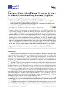
However, even in a case when a measurement model includes a prediction error, there could still be some gain. Generally, in order to get any gain, the error value should be smaller than a sum of the prediction fuzziness and the measurement errors. This relationship allows a model maker to develop a strategy that avoids any loss. If a model maker X confident about the prediction value, a fuzzy prediction ~ ~ −1 T T −1 T −1 T −1 T −is EX~ = M[(X − X )(X − X ) ] = ( A Σ y A + 2B Σb B) (4B Σb ( f − BX)( f − BX) Σb1B model with a low prediction fuzziness should be applied and + AT Σ−y1 A)(AT Σ−y1 A + 2BT Σb−1B)−1 ; a high gain could be achieved. However, when the confidence level decreases, the prediction fuzziness could be The problem of this gain evaluation deserves special increased, which avoids losses but might make the gain consideration. To evaluate the gain provided by an expert’s value lower . information application, let us choose the projection of the estimate’s MSE, which can be written as Sensor networks example. Sensor networks, which 1 converge the Internet, communications, and information T = Tr ( E Xˆ E X−~1 ) = K technologies with miniaturization techniques, have provided 1 T −1 −1 T −1 T −1 T −1 T −1 T −1 −1 new opportunities for acquiring and communicating huge Tr[(A Σy A) (A Σy A+ 2B Σb B)(4B Σb ( f − BX)( f − BX) Σb B + A Σy A) K arrays of information coming from heterogeneous sensors ( AT Σ −y1 A + 2 B T Σ b−1 B )] and sensor arrays. The Wireless Sensor Network (WSN) where K is the number of measured research platform used in this research includes the TelosB variables. Berkeley Motes which were originally manufactured by The gain depends on the measurement system structure CrossBow Technologies Inc. In this example we consider an and errors, as well as prediction model errors and its application of motes, each of which includes three sensors: uncertainty factors (actually the ratio between the prediction illumination, temperature and humidity. Humidity and error to the fuzziness). Fig. 1 demonstrates that the change in temperature sensors readings can be converted to SI units as the gain value depends on the uncertainty prediction factor follows: for temperature readings, Oscilloscope (software (prediction interval) or actually on the prediction fuzziness utility used in this project to collect and transmit when the mean measurement error is fixed and prediction measurement results) returns a 14-bit value that can be errors. The plots were constructed by computer simulation converted to degrees Celsius according to the formula: for four different cases of measurement distributions and t Tc = −39.60 + 0.01* S t , where S is the raw output of the prediction types studied in this paper. The maximum gain sensor. Humidity is a 12-bit value that is not temperature could be achieved when the prediction is absolutely accurate compensated and is calculated according to the formula: (prediction error is zero). One can see that with an increase rh H = −4.0 + (0.0405* S rh ) + (−2.8 *10−6 )(S rh ) 2 , where S is the in prediction errors, the gain goes down and transforms into raw output of the relative humidity sensor. One can loss when the error in prediction becomes considerably determine the true humidity (with temperature larger than its fuzziness. This gain/loss transformation is compensation) by using the following calculation: more dramatic in the cases of normal measurement We humidity true = (Tc − 25)[0.01+ (0.00008 * S rh )] + H . distribution in comparison to the uniform one. However, conducted experiments with up to four motes, measuring with uniform distribution, the maximum gain value is also temperature and humidity indoors (college building, student much smaller. dorm). The temperature measurements vary in 6 -7 bits, producing a measurement error of up to 110 sensor units. IV. PRACTICAL RECOMMENDATIONS AND EXAMPLES OF These measurement errors could be substituted into formula THE PREDICTION MODEL APPLICATION IN MEASUREMENT (1), where the matrix A is composed of the coefficients (WHAT GAIN COULD BE ACHIEVED WITH A RATHER calculated from the above graduation parameters and the INACCURATE MEASUREMENT MODEL?) measurement scheme applied. However, assuming that the The typical measurement accuracy for the modern multimeasurements of different sensors are not correlated as they channel sensor systems could be in the vicinity of 1-2%. In a were received from different motes, we may recalculate the case of 2% measurement error with a prediction fuzziness of measurement errors in degrees, which will be 1.1 degree and 20%, which is rather high, could achieve the gain up to 44%. apply it to all four sensors. Let us suppose that an expert may An example of a reasonable practical prediction might be give the approximate value temperature prediction with a like “the measured variable has a value of around 10 units or prediction interval up to +/- 5 degrees. Fig. 2 gives the
calculation result of a possible gain from the application of an expert’s prediction and presents the possible gain area with four sensors measuring and transmitting the temperature. One can see that, with a rather high confidence (the prediction fuzziness is about one degree), one can achieve a gain in accuracy of up to 50% under the condition that the prediction is accurate. Here the prediction error should be less than one degree, otherwise the loss will occur. However, widening the prediction fuzziness to about five degrees will allow tolerating prediction errors of up to three degrees. V.
sensor readings can be fused with data from alternate sources to result in accuracy gains. Historical sensor data, expertsupplied domain knowledge, technical information about the sensors, fuzzy logic, and other methods can be combined to develop a measurement model. When a correctly generated measurement model is applied to sensor network data, the accuracy of the results can be significantly improved. REFERENCES [1]
L. Reznik, G. Solopchenko Use of a priori Information on Functional Relations between Measured Quantities for Improving Accuracy of Measurement. MEASUREMENT, 1986, v.3, 2, pp.61-69
CONCLUSION
Conventional measurement methods used in sensor networks can be significantly improved through the introduction of a complex object measurement model. The
Figure 1. Dependence of the gain (level bigger than 1)/loss (level lower than 1) on the model error and the model uncertainty factor (prediction errors and intervals are scaled in measurement error units), case A: uniform distribution of the measurements and interval model, case B: normal distribution of the measurements and interval model, case C: uniform measurements distribution and approximate value model, case D: normal measurements distribution and approximate value prediction – received by computer simulation
Figure 2. Dependence of the possible gain/loss on the model error and the model uncertainty as well as the area where the gain could be achieved – received from real experiments with the sensor network built from four Telos ver. B motes produced by Crossbow Technologies Inc.