improving artificial neural network performance in calibrating doubly ...

IMPROVING ARTIFICIAL NEURAL NETWORK PERFORMANCE IN CALIBRATING DOUBLYCONSTRAINED WORK TRIP DISTRIBUTION BY USING A SIMPLE DATA NORMALIZATION AND LINEAR ACTIVATION FUNCTION Gusri Yaldi1, M A P Taylor2, Wen Long Yue3 1 PhD Candidate, ISST-Transport Systems, University of South Australia 2 Director, Institute for Sustainable Systems and Technologies, University of South Australia 3 Senior Lecturer, Program Director, ISST-Transport Systems, University of South Australia ABSTRACT The applications of Artificial Neural Networks (NN) in estimating work trip distribution is a unique case study as its performance is not only measured in term of the error level in the estimated trips, but also by its ability to satisfy the Production and Attraction constraints. Previous research indicated that NN models were unable to fulfil those constraints and had rather poor generalization ability. However, this study has indicated that a NN with simple data normalization and a linear activation function (Purelin) in the output layer could accomplish the two constraints, with average correlation coefficients (r) of 0.958 and 0.997 for Production and Attraction respectively. The test results have also provided evidence that a validated NN could provide a similar goodness of fit as a doubly-constrained gravity model. However, the error level is still higher than the gravity model as indicated by the average Root Mean Square Error (RMSE), where the RMSE for the NN and Gravity Model are 181 and 174 respectively. Finally, the study suggests that the NN can be used to calibrate doublyconstrained trip distribution matrices; although, further study and refinement is required to improve the model’s performance. Keyword: Data Normalization, Activation Function, Work Trip

1. INTRODUCTION The success of a transportation planning study is dependent upon many factors. One of them is the existence of a reliable supporting data set. Among the data itself, the Origin and Destination work trip data is of particular importance because the trend of future trip flow can be predicted. As transport development impacts can cover multidimensional aspects of life such as society, the environment and the economy, the trip distribution data must have acceptable levels of accuracy and precision. A robust and efficient technique is required to predict the patterns of trips in the future, so that the desired outcomes and impacts can be achieved and anticipated. There is no technique in trip distribution that is universally applicable, so attempts to develop alternative ways are always needed. This includes the adoption of approaches from other disciplines. Neural Networks are one of them and are proposed as an alternative method in this study. The use of NN in modelling activities is growing fast and covers many disciplines, including transport systems. The literature suggests that NN were used in some 13 categories of transport studies up to year 1990 where driver behaviour simulation models had the highest percentage of NN applications (Dougherty, 1995). However, more recent investigation nd

32 Australasian Transport Research Forum

1

indicates a growing adoption of NN in travel demand modelling, dominated by Mode Choice and Trip Distribution. An approach must be supported by logic and sensible underpinning theory, and without it NN is just a naive computational tool. According to Black (1995), NN is an intelligent computer system that mimics the processing capabilities of the human brain. It is a forecasting method that specifies output by minimizing an error term indicated by the deviation between input and output through the use of a specific training algorithm and random learning rate (Black, 1995; Zhang et al, 1998). Various studies in transportation provide evidence of the advantages and disadvantages of using NN. It is usually compared with the existing methods in relevant studies. For example, the multilayer perceptron neural network has been compared with the Discrete Choice Model (DCM) for mode choice study as reported by Cantarella & de Luca (2005), Hensher & Ton (2000), Carvalho et al. (1998), and Subba Rao et al. (1998). There is less application of NN in trip distribution compared to mode choice studies. Black (1995) reported a study of spatial interaction modelling using NN focusing on commodity flows. This model was structured similarly to the doubly constrained gravity model (DCGM) and named as the Gravity Artificial Neural Network (GANN). For passenger flow modelling, Mozolin et al. (2000) used NN to model trip distribution, also characterized by DCGM. The studies by Black and Mozolin et al. were also multilayer perceptron neural networks. NN is characterized by its important properties, such as learning algorithm, activation function, number of layers, number of nodes inside each layer, and learning rate (Teodorovic and Vukadinovic, 1998, Dougherty, 1995). The amount of data and the split of the data used for training, validating and testing is also important for NN fitting performance (Carvalho et al., 1998). Zhang et al. (1998) suggested that in the absence of proper guidelines, NN model development can only be done through trial and error procedures. There is also a lack of reported studies on the behaviour of NN with regard to these properties. Lack of knowledge in defining the main properties of NN could lead to disadvantages in using this artificial intelligent approach, for example if the modeller is unable to enforce the network to behave according to the required constraints. This happened in the study by Mozolin et al. (2000). They reported that NN was unable to meet the double constraints and they used adjustment factors for the output of the NN so that it met the Production and Attraction constraints. They also reported that NN had rather poor generalization ability. Although this was not comprehensively discussed, Black (1995) presented a small report about the same issue in commodity flow estimation using NN. It was not clear whether the model can properly satisfy the constraints. This study aims at meeting the Production and Attraction constraints and improving the generalization ability by looking more intensively in the selection of the activation function and data normalization methods. There appears to be little research until recently on the relative performance of using difference activation functions, including a combination of linear and non-linear activation functions. Therefore, the effects of different activation functions toward the performance of the networks have not been previously investigated. nd

32 Australasian Transport Research Forum

2

Meanwhile, Zhang et al. (1998) suggested that a linear transfer function is practical for use in forecasting, especially when the targets involve continuous values. However, the previous research merely used the same activation functions between hidden and output layers, and used the logistic function to capture the nonlinearity between input and output data. Thus, a study that investigates the impact of different activation functions toward the network performance could be a significant contribution to this approach development. This study focuses on passenger trip distribution, especially work trips. The Neural Networks are categorized into two grand scenarios, termed Norm 1 and Norm2. Norm1 and Norm2 are used to asses the ability of the NN in fulfilling the constraints based on different data normalization methods. Norm1 is also used in testing the generalization ability of the NN to predict the work trips. Neural Networks with a constant number of ten nodes in the hidden layer were trained and validated. Different activation functions between hidden and output layers were used, which seems not to have been done before. Comparisons with the doubly constrained gravity model (DCGM) were used to measure the generalization ability of NN models.

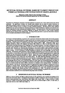
2. MODEL DEVELOPMENT AND METHODOLOGY The models are developed using the structure as illustrated by Figure 1. This has three input nodes representing the Trip Production (Pi), Trip Attraction (Aj) and Distance (Dij). There is one node in the output layer, the estimated trip number (Tij). Each node is connected to the hidden layer nodes by connection weights wj-i and wk-j. The work trip data is based on the 2005 home interview survey conducted in Padang City, West Sumatra, Indonesia. This includes 36 zones. Two data normalization methods are used in this study, namely simple and statistical normalizations. Simple normalization will convert the input data to the range [0, 1]. The statistical normalization will convert the input data based on its mean and standard deviation. Matlab 7.0.1 is used to develop the network, where the initial connection weights are randomly defined by the tool. To investigate the network ability to fulfil the Production and Attraction constraints, the network is trained with whole data. To avoid over-fitting, the training is limited to 100 epochs. Over-fitting may still occur, however, this will not affect its generalization ability since the testing is not undertaken yet at this stage. The objective here is only to examine the Production and Attraction output generated by the network.

Figure 1 The Network Topography nd

32 Australasian Transport Research Forum

3

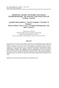
Meanwhile, the second category of the network is aimed at examining the generalization ability of the network. In order to avoid over-fitting, the network can be validated so that the training is stopped when the error in the validation network starts to increase (Zhang et al., 1998). Therefore, there is also validation and testing in addition to the training. 40 per cent of the whole data is used to train the model, 30 per cent is used to validate the model and the other 30 per cent is used to test it. The data set members are randomly selected without replacement. The training is limited to 100 epochs. NN is a forecasting method based on the functions of the human brain in processing perceived information. There is no objective mathematical formulation used in each node, except the summation in the hidden and output layer nodes. The summation in the hidden layer is to add together the results of multiplications between the inputs and the connection weights connecting them. Meanwhile, the summation in the output node is to add together the results of multiplications of summation in the hidden layer nodes and the weights connecting them with the output nodes. Then, the results are compared with the actual ones. If the difference is above the limit, the connection weights are adjusted based on that error which is back propagated to the network. The adjustment is conducted based on the Marquardt-Lavenberg algorithm for nonlinear least squares (Hagan and Menhaj, 1994). There are four common activation functions according to Teodorovic and Vukadinovic (1998), and two of them are Sigmoid and Linear functions. Sigmoid functions have often been used in different transportation studies, such as the studies by Mozolin et al. (2000), Carvalho et al. (1998), and Black (1995). Although the activation function is one of the main properties of the NN, there is no study specifically reporting the use of different activation functions and their impact on the network performance. Three activation functions are used and combined in this study. They are the Tansig, Logsig and Purelin functions. The mathematical formulations of these functions are given below. 1. Tansig

(1)

2. Logsig

(2)

3. Linear

(3)

1

1

1 0

0

(a)

(b)

0 -1

-1

(c)

Figure 2 Common Activation Function

The first and second activation functions will squeeze the summation results in each node of the hidden and output layers based on the graphs depicted by Figure 2. The Tansig function will give results in the range [-1, 1] and for Logsig in [0, 1]. Meanwhile, the linear transfer function will not change the summation results and just transfers them after the summation process, and hence the outputs have no limits. With this knowledge, the selection of the

nd

32 Australasian Transport Research Forum

4

activation function and the data normalization is a crucial decision. The following factors are considered in selecting the activation function: 1. The activation functions in the hidden layer must be able to capture the nonlinearity between input and output 2. Different activation functions can be used in the hidden and output layers 3. Due to all the data being positive, the activation in the hidden layer must not allow the summation outputs to be negative values 4. The activation functions in the output layer merely summarize the results from previous layer, and hence the nonlinearity between output and input is only captured in the hidden layer 5. The activation function in the output layer must ensure it does not generate negative outputs (estimated trips) Based on the explanations above, Logsig is a suitable activation function in the hidden layer. For the output layer, Purelin is then considered the most suitable function for forecasting the trip numbers. However, other activation functions will be also used in the output nodes in order to see their impacts on the average network performance. Details are given in Table 1. Table 1 Scenario Norm1

Norm2

Network Scenarios Activation function Data Hidden Output normalization Layer Layer xi = xo/xmax Logsig Purelin Logsig Logsig Logsig Tansig Purelin xi = (xo- x)/SD Logsig

Number of experiment 10 times

Data Input nodes

Output Node

Trip Production Trip Attraction Distance

Observed Trip

Due to the random /stochastic nature of the initial weights selection, each training will result in different outputs and performance. Therefore, the training is conducted ten times, and then the average performance is used at the final measurements. Firstly, the network is trained with the whole data for both grand scenarios (Norm1 and Norm2) which have the Logsig and Purelin activation functions in the hidden and output layers. The purpose is to define the impact of different data normalization methods (Norm1 and Norm2) to the accomplishment of constraints based on the correlation coefficient (r) between the estimated and observed Production and Attraction. After that, the impacts of different activation functions, but the same data normalization (Norm1) are investigated through modification in grand scenario Norm1, as can be seen in the Table 1. The independent t-test is used to evaluate the significance of the difference in the average performance between each grand scenario in terms of the average Root Mean Square Error (RMSE) and correlation coefficient (based on Fisher’s Z transformation). The paired t-test is used within the Norm 1 scenario, to investigate the significance level of the change in the average performance before and after modification (Logsig-Purelin, Logsig-Logsig, LogsigPurelin). The Fisher’s Z transformation is used to conduct the statistic test for r. Meanwhile, an independent 2-test is used to test the variation within each scenario. nd

32 Australasian Transport Research Forum

5

The best scenario is then compared with the doubly-constrained gravity model calibrated using Hyman’s maximum likelihood algorithm (Hyman, 1969). The generalization ability of the network in term of relative performance to predict the trip numbers are defined based on two categories, namely the error level (RMSE) and the ability to predict the trend (r). Finally, independent t, Fisher’s Z, and 2-tests are conducted to measure the testing performance of the NN compared to the Gravity model.

3. DATA OUTPUT ANALYSIS The result of each training is reported in Tables 2, 3, 4 and 5. Table 2 contains the results of the training of grand scenarios Norm1 and Norm2 as described in the previous section. It can be seen that the two scenarios with the same activation functions in hidden and output layers (Logsig-Purelin) generate different figures (r), especially for the Production constraint. The Norm1 scenario is able to satisfy both constraints. In addition, the NN model can fulfil the Attraction constraint with higher correlation coefficient than the Production constraint. The average r for Production (rP) is 0.958 and 0.816 for Norm1 and Norm2 respectively. The 2 -test suggests that variations between each experiment within the same scenario are not significant for both grand scenarios. Then, Norm1 has a significantly higher rP than Norm2 as tested statistically using Fisher’s Z transformation for the correlation coefficient. Both scenarios have an average r for attraction (rA) that is above 0.99, and the difference between them is not significant. The test results also suggest that the first grand scenario has a significantly higher performance in term of level of error (RMSE) and correlation coefficient (rT) between estimated and observed trips. It can be concluded that when the data is normalized to its maximum value, the neural network can fulfil both constraints satisfactorily. Table 2 Mean and Variance test for Norm1 and Norm2 Trial 1 2 3 4 5 6 7 8 9 10 Mean 2 test t- test

Norm1 rP 0.955 0.965 0.948 0.951 0.957 0.964 0.958 0.959 0.960 0.964 0.958 1.354 (19.02) 3.460 (2.009)

rA 0.996 0.996 0.996 0.996 0.997 0.997 0.997 0.997 0.997 0.996 0.997 1.564 (19.02) -0.070 (2.009)

rT 0.846 0.836 0.845 0.846 0.842 0.841 0.837 0.839 0.848 0.843 0.842 2.258 (19.02) 2.315 (1.96)

RMSE 157 161 157 157 159 159 161 160 156 158 159

Norm2 rP 0.819 0.829 0.790 0.803 0.820 0.808 0.838 0.826 0.811 0.814 0.816 0.502 (19.02)

rA 0.997 0.998 0.997 0.996 0.997 0.997 0.996 0.997 0.996 0.997 0.997 2.880 (19.02)

rT 0.812 0.81 0.805 0.819 0.814 0.811 0.826 0.811 0.811 0.818 0.814 3.613 (19.02)

RMSE 172 172 175 169 171 172 166 172 172 169 171

13.23 (2.262)

Although the Norm1 with Logsig and Purelin activation functions in hidden and output layers can fulfil both constraints satisfactorily, some of the outputs (the estimated trips) have negative values. This arises because the activation function in the output layer does not squeeze the summation to the same interval as the input data. This is not the same as the real data, where there are no negative trips. Thus, the activation function in the output layer nd

32 Australasian Transport Research Forum

6

is switched to Logsig which will squeeze the output within the range [0, 1]. The weakness of this function when used in the output layer is that it squeezes the output non-linearly (see Figure 2b). Tansig is also used in the output layer, and its weakness when used in the output layer is the same as Logsig. However, it transfers the output within the range [-1, 1]. This could level up its performance. The results of these trials are reported in Table 3. Table 3 Mean and Variance Tests for Grand Scenario Norm1 for the Correlation Coefficient (r) Trial 1 2 3 4 5 6 7 8 9 10 Mean 2 test

LogsigTansig rP 0.962 0.966 0.962 0.962 0.940 0.966 0.963 0.946 0.947 0.967 0.958

rA 0.996 0.997 0.997 0.996 0.996 0.997 0.996 0.996 0.995 0.997 0.996

LogsigLogsig rP 0.955 0.937 0.956 0.959 0.938 0.927 0.950 0.956 0.958 0.945 0.948

rA 0.995 0.995 0.996 0.996 0.996 0.995 0.997 0.996 0.996 0.995 0.996

Fisher’s Z-transformation test

LogsigPurelin rP 0.955 0.965 0.948 0.951 0.957 0.964 0.958 0.959 0.960 0.964 0.958

rA 0.996 0.996 0.996 0.996 0.997 0.997 0.997 0.997 0.997 0.996 0.997

LogsigTansig zP 1.969 2.027 1.973 1.969 1.734 2.026 1.983 1.792 1.806 2.039 1.932 3.669 (19.02) -0.043 (2.02)

zA 3.047 3.234 3.250 3.132 3.082 3.188 3.145 3.082 3.005 3.188 3.135 1.951 (19.02) 0.294 (2.02)

LogsigLogsig zP 1.8903 1.7137 1.8938 1.9371 1.7245 1.6388 1.8318 1.8926 1.9247 1.7810 1.8228 3.140 (19.02) 0.583 (2.02)

zA 2.9653 3.0255 3.1190 3.1190 3.0819 2.9653 3.1732 3.1454 3.1063 2.9846 3.0685 1.774 (19.02) 0.678 (2.02)

LogsigPurelin zP 1.886 2.008 1.810 1.838 1.905 2.001 1.919 1.936 1.946 1.995 1.924 1.354 (19.02)

zA 3.132 3.106 3.159 3.132 3.250 3.234 3.285 3.285 3.188 3.094 3.187 1.564 19.02)

The results suggest that both Tansig and Purelin when being used in the output layer have very similar correlation coefficients; however, the variance is higher for Tansig than Purelin. The variation within each scenario is measured again by using the 2-test. It can be seen in Table 3 that the variation is not significant, where Logsig-Purelin has the lowest 2 values. Then, a paired two-tailed t-test based on Fisher’s Z transformation with a level of confidence ( ) of 0.05 shows that the modified scenarios perform at the same level as the base scenario (Logsig-Purelin). If the performance of the modification is compared to each other, then the Logsig-Tansig scenario is better than Logsig-Logsig scenario in term of average correlation coefficient. The Logsig-Tansig scenario allows the output to be outside the range [0, 1], but still in the range [-1, 1]. This indicates that the linear function in output layer (Logsig-Purelin) is more suitable for forecasting the trip numbers than others. Therefore, the ranking of the best performance is as follows: 1. Logsig-Purelin 2. Logsig-Tansig 3. Logsig-Logsig However, using a linear function in the output layer also has weaknesses. The outputs can be negative values, and this is against the reality where there is no such negative trip. The number of negative outputs is about five per cent of the whole data (1296 samples). Among that five per cent sample, more than 95 per cent has its original value of zero (no trip). In dealing with this case and finding, a modification is applied to the estimated trips. The modification is intended to remove the negative outputs, yet, the performance should remain constant. In adjusting the output of the network, the following conditions are applied. (4) nd

32 Australasian Transport Research Forum

7

Thus, the negative value trip is replaced by zero. As the negative outputs belong to the zone where there was no trip, removing negative values will not change the performance significantly. The average r for Production is slightly changed than before modification; however, it is not statistically significant. Therefore, this approach is acceptable. Finally, the performance of the Norm1 scenario is compared with the doubly-constrained gravity model. The comparison is conducted at two levels, calibration and testing (generalization ability). The results are reported in Tables 4 and 5. The results suggest that the calibration performance for all scenarios in Norm1 outperforms the Gravity’s Model as the error level is significantly lower, while the correlation coefficient is significantly higher. Table 4 Comparison between Norm1 Scenario and Gravity Models (Calibration) RMSE Correlation Coefficient (r) Trial Logsig-Tansig Logsig-Logsig Logsig-Purelin Logsig-Tansig Logsig-Logsig 1 160 159 157 0.839 0.842 2 164 153 161 0.831 0.855 3 160 159 157 0.839 0.842 4 161 159 157 0.838 0.841 5 153 154 159 0.854 0.853 6 163 155 159 0.832 0.851 7 160 160 161 0.839 0.839 8 157 159 160 0.846 0.841 9 159 159 156 0.841 0.841 10 162 158 158 0.836 0.844 Mean 160 158 159 0.840 0.845 Gravity’ RMSE = 168; r= 0.822 2 6.126(19.02) 4.918(19.02) t- test -8.149(1.960) -13.25(1.960) -16.881(1.960) 2.013(1.960) 2.679(1.960) Table 5 Comparison between Norm1 Scenario and Gravity Models (Testing) RMSE Correlation Coefficient (r) Trial LogsigLogsigLogsigLogsig-Tansig Logsig-Logsig Tansig Logsig Purelin 1 170 184 175 0.819 0.786 2 212 185 176 0.769 0.796 3 168 176 178 0.829 0.805 4 174 176 194 0.809 0.807 5 171 180 181 0.816 0.800 6 181 187 179 0.795 0.801 7 196 173 191 0.762 0.812 8 173 181 177 0.814 0.817 9 173 171 180 0.813 0.821 10 176 174 175 0.809 0.811 Mean 179 179 181 Gravity’ RMSE = 174; r= 0.827 2 12.293(19.02) 3.071(19.02) t-test 1.307(1.960) 3.054(1.960) 3.31(1.960) -1.349(1.960) -1.273(1.960)

Logsig-Purelin 0.846 0.836 0.845 0.846 0.842 0.841 0.837 0.839 0.848 0.843 0.842 2.258(19.02) 2.348(1.960)

Logsig-Purelin 0.809 0.811 0.806 0.757 0.793 0.805 0.804 0.807 0.804 0.813

6.293(19.02) -1.526(1.960)

The gravity model has a statistically better performance in term of Root Mean Square Error (RMSE) than the neural network at the testing level, except for the Logsig-Tansig scenario. However, that scenario has the highest variation in the correlation coefficient than others. Then, both models have almost the same ability in predicting the trend or the pattern of the nd

32 Australasian Transport Research Forum

8

trip number distribution as indicated by the value of r. It can be concluded that for this data set the NN model can calibrate the trip matrix better than the gravity model suggested by the calibration results. It can predict the trend at the same level as the gravity model, but with higher discrepancy between estimated and observed trips. In order words, neural network can calibrate the trip matrix, with the result closer to the distribution of the base trip matrix; however, the error is slightly higher than the Gravity model when predicting the trip as indicated by the test results.

4. CONCLUSIONS AND FURTHER STUDIES Based on the results of the experiment as explained in the preceding sections, it can be concluded that the Neural Network model can be used to calibrate and to forecast trip distribution, especially for work trips. It is able to accomplish the Production and Attraction constraints satisfactorily. Neural Network is also able to estimate the work trip number distribution. The correlation coefficients between estimated and observed trips are statistically the same. However, the discrepancy between estimated and observed trips is still higher than those found for the gravity model. Further attention must be devoted in selecting the activation function as well as the normalization methods. The research indicates that normalizing the data to its maximum value is more appropriate in calibrating the models as indicated by this NN model’s ability to satisfy the constraints, which is higher than the statistical normalization method. It also suggests that the linear activation function is more suitable in the output layer than nonlinear functions for calibration purposes. Further studies will involve using other method in normalizing the input data. Based on the findings in this research, non-linear data transformation could further improve the testing performance of the Neural Network. It is due to the input data will be nonlinearly transformed, including the target values (tij). Thus, the error computation will be based on the deviation between the NN model outputs (tij), which are nonlinearly transformed by the Tansig or Logsig function, and the target values (Tij) which are also transformed nonlinearly by using Tansig or Logsig functions.

5. REFERENCES BLACK, W. R. (1995) Spatial interaction modeling using artificial neural networks. Journal of Transport Geography, 3, 159-166. CANTARELLA, G. E. & DE LUCA, S. (2005) Multilayer feedforward networks for transportation mode choice analysis: An analysis and a comparison with random utility models. Transportation Research Part C: Emerging Technologies, 13, 121-155. CARVALHO, M. C. M., DOUGHERTY, M. S., FOWKES, A. S. & WARDMAN, M. R. (1998) Forecasting travel demand: a comparison of logit and artificial neural network methods. The Journal of the Operational Research Society, 49, 711-722. DOUGHERTY, M. (1995) A review of neural networks applied to transport. Transportation Research Part C: Emerging Technologies, 3, 247-260. nd

32 Australasian Transport Research Forum

9

HAGAN, M. T. & MENHAJ, M. B. (1994) Training feedforward networks with the Marquardt algorithm. Neural Networks, IEEE Transactions on, 5, 989-993. HENSHER, D. A. & TON, T. T. (2000) A comparison of the predictive potential of artificial neural networks and nested logit models for commuter mode choice. Transportation Research Part E: Logistics and Transportation Review, 36, 155-172. HYMAN, G. M. (1969) The Calibration of Trip Distribution Models. Environment and Planning, 1, 105112. MOZOLIN, M., THILL, J. C. & LYNN, U. E. (2000) Trip distribution forecasting with multilayer perceptron neural networks: A critical evaluation. Transportation Research Part B: Methodological, 34, 53-73. SUBBA RAO, P. V., SIKDAR, P. K., KRISHNA RAO, K. V. & DHINGRA, S. L. (1998) Another insight into artificial neural networks through behavioural analysis of access mode choice. Computers, Environment and Urban Systems, 22, 485-496. TEODOROVIC, D. & VUKADINOVIC, K. (1998) Traffic Control and Transport Planning: A Fuzzy Sets and Neural Networks Approach, Massachusetts, USA, Kluwer Academic Publisher. ZHANG, G., PATUWO, B. E. & HU, M. Y. (1998) Forecasting with artificial neural networks:: The state of the art. International Journal of Forecasting, 14, 35-62.

nd

32 Australasian Transport Research Forum

10