The complete code of the robust tracker is available via ftp. Keywords: Feature tracking; Motion analysis; Optical flow; Registration; Robust statistics; X84. 1.
Pattern Analysis & Applications (1999)2:312–320 1999 Springer-Verlag London Limited
Improving Feature Tracking with Robust Statistics A. Fusiello1, E. Trucco2, T. Tommasini1, V. Roberto1 1
Dipartimento di Matematica e Informatica, Universita` di Udine, Udine, Italy; 2Department of Computing and Electrical Engineering, Heriot-Watt University, Edinburgh, UK
Abstract: This paper addresses robust feature tracking. The aim is to track point features in a sequence of images and to identify unreliable features resulting from occlusions, perspective distortions and strong intensity changes. We extend the well-known Shi–Tomasi–Kanade tracker by introducing an automatic scheme for rejecting spurious features. We employ a simple and efficient outliers rejection rule, called X84, and prove that its theoretical assumptions are satisfied in the feature tracking scenario. Experiments with real and synthetic images confirm that our algorithm consistently discards unreliable features; we show a quantitative example of the benefits introduced by the algorithm for the case of fundamental matrix estimation. The complete code of the robust tracker is available via ftp. Keywords: Feature tracking; Motion analysis; Optical flow; Registration; Robust statistics; X84
1. INTRODUCTION Much work on structure from motion [1] has assumed that correspondences through a sequence of images could be recovered. Feature tracking finds matches by selecting image features and tracks these as they move from frame to frame. It can be seen as an instance of the general problem of computing the optical flow, that is, the vector’s field that describes how the image is changing with time, at relatively sparse image positions [2–4]. Methods based on the detection of two-dimensional features (such as corners) have the advantage that the full optical flow is known at every measurement position, because they do not suffer from the aperture problem effect (a discussion on this subject can be found elsewhere [5]). Work on tracking two-dimensional features can be found elsewhere [6–10]. Robust tracking means automatically detecting unreliable matches, or outliers, over an image sequence (see elsewhere [11] for a survey of robust methods in Computer Vision). Recent examples of such robust algorithms include reference 12, which identifies tracking outliers while estimating the fundamental matrix, and reference 13, which adopts a RANSAC [14] approach to eliminate outliers for estimating the Received: 22 January 1999 Received in revised form: 3 May 1999 Accepted: 3 May 1999
trifocal tensor. Such approaches increase the computational cost of tracking significantly, as they are based on the robust estimation of 3D motion via iterative algorithms. Black and Jepson [15] describe a method for tracking objects using eigen-representations. The matching between the eigenspace (which represents the object) and the image is done using robust regression. This paper concentrates on the well-known Shi–Tomasi– Kanade tracker, and proposes a robust version based on an efficient outlier rejection scheme. Building on results from Lucas and Kanade [6], Tomasi and Kanade [16] introduced a feature tracker based on SSD matching and assuming translational frame-to-frame displacements. Subsequently, Shi and Tomasi [17] proposed an affine model, which proved adequate for region matching over longer time spans. Their system classified a tracked feature as good (reliable) or bad (unreliable) according to the residual of the match between the associated image region in the first and current frames; if the residual exceeded a user-defined threshold, the feature was rejected. Visual inspection of the results demonstrated good discrimination between good and bad features, but the authors did not specify how to reject bad features automatically. This is the problem that our method solves. We extend the Shi–Tomasi–Kanade tracker (Section 2) by introducing an automatic scheme for rejecting spurious features. We employ a simple, efficient outlier rejection rule, called X84,
Improving Feature Tracking with Robust Statistics
313
and prove that its assumptions are satisfied in the feature tracking scenario (Section 3). Our robust tracking algorithm is summarised in Section 4. Experiments with real and synthetic images confirm that our algorithm makes good features track better, in the sense that outliers are located reliably (Section 5). We illustrate quantitatively the benefits introduced by the algorithm with the example of fundamental matrix estimation. Image sequences with results and the source code of the robust tracker are available on-line (http://www.dimi.uniud.it/ ˜fusiello/demo-rtr/).
2. SHI–TOMASI–KANADE TRACKER In this section the Shi–Tomasi–Kanade tracker [17,16] will be briefly described. Consider an image sequence I(x,t), where x ⫽ [u,v]ⳕ are the coordinates of an image point. If the time sampling frequency (that is, the frame rate) is sufficiently high, we can assume that small image regions undergo a geometric transformation, but their intensities remain unchanged: I(x,t) ⫽ I(␦(x),t ⫹ )
(1)
where ␦(·) is the motion field, specifying the warping that is applied to image points. The fast-sampling hypothesis allows us to approximate the motion with a translation, i.e.
␦(x) ⫽ x ⫹ d
(2)
where d is a displacement vector. The tracker’s task is to compute d for a number of automatically selected point features for each pair of successive frames in the sequence. As the image motion model is not perfect, and because of image noise, Eq. (1) is not satisfied exactly. The problem is then finding the displacement d which minimises the SSD residual
⑀⫽
冘
[I(x ⫹ d,t ⫹ ) ⫺ I(x,t)]2
C⫽
冘冋 冘 W
I2u
IuIv
IuIv
I2v
g⫽⫺
册
(7)
It[IuIv]ⳕ
(8)
W
If dk ⫽ C⫺1g is the displacement estimate at iteration k, and assuming a unit time interval between frames, the algorithm for minimising (5) is the following:
冦
d0 ⫽ 0 dk⫹1 ⫽ dk ⫹ C⫺1
冘冋
册
(I(x,t) ⫺ I(x ⫹ dk,t ⫹ 1)) ⵜI(x,t)
W
2.1. Feature Extraction
A feature is defined as a region that can be tracked easily from one frame to the other. In this framework, a feature can be tracked reliably if a numerically stable solution to Eq. (6) can be found, which requires that C is wellconditioned and its entries are well above the noise level. In practice, since the larger eigenvalue is bound by the maximum allowable pixel value, the requirement is that the smaller eigenvalue must be sufficiently large. Calling 1 and 2 the eigenvalues of C, we accept the corresponding feature if min(1,2) ⬍ t
(9)
where t is a user-defined threshold [17]. This algebraic characterisation of ‘trackable’ features has an interesting interpretation, as they turn out to be corners, that is, image features characterised by an intensity discontinuity in two directions. Since the motion of an image feature can be measured only in its projection on the
(3)
W
where W is a given feature window centred on the point x. In the following we will solve this problem by means of a Newton–Raphson iterative search. Thanks to the fast-sampling assumption, we can approximate I(x ⫹ d,t ⫹ ) with its first-order Taylor expansion: I(x⫹d,t⫹) ⬇ I(x,t) ⫹ ⵜI(x,t)ⳕd⫹It(x,t)
(4)
where ⵜIⳕ ⫽ [Iu,Iv] ⫽ [⭸I/⭸u,⭸I/⭸v] and It ⫽ ⭸I/⭸t. We can then rewrite the residual (3) as
⑀⬇
冘
(ⵜI(x,t)ⳕd ⫹ It(x,t))2
(5)
W
To minimise the residual (5), we differentiate it with respect to the unknown displacement d and set the result to zero, obtaining the linear system Cd ⫽ g where
(6)
Fig. 1. Value of min(1,2) for the first frame of ‘Artichoke’. Window size is 15 pixels. Darker points have a higher minimum eigenvalue.
314
A. Fusiello et al.
brightness gradient (aperture problem), corners are the features whose motion can be measured. Discontinuity can be detected, for instance, using normalised cross-correlation, which measures how well an image patch matches other portions of the image as it is shifted from its original location. A patch which has a well-defined peak in its auto-correlation function can be classified as a corner. Let us compute the change in intensity as the sum of squared differences in the direction h for a patch W centred in x ⫽ (u,v):
冘
Eh(x) ⫽
I(x ⫹ d) ⫺ I(x ⫹ d ⫹ h)2
(10)
accounting for affine warping, and can be written as M ⫽ 1 ⫹ D, with D ⫽ (dij] a deformation matrix and 1 the identity matrix. Similar to the translational case, one estimates the motion parameters, D and d, by minimizing the residual
⑀⫽
冘 冘 冘 冉 冉冘冋
Eh(x) ⬇
(ⵜI(x ⫹ d)ⳕh)2
Bz ⫽ f,
in which z ⫽ [d11 d12 d21 d22 d1 d2]ⳕ contains the unknown motion parameters, and
冘
h (ⵜI(x ⫹ d))(ⵜI(x ⫹ d)) h ⳕ
d苸W
⫽
hⳕ
d苸W
⫽h
ⳕ
d苸W
I2u
IuIv
IuIv
2 v
I 2 u
冊
I
IuIv
IuIv
I2v
h
册冊
It[uIu uIv vIu vIv Iu Iv]T
W
B⫽
(11)
冘冋 W
U
V
ⳕ
C
V
册
with h
The change in intensity around x is therefore given by Eh(x) ⫽ hⳕ C h
1 ⬍ Eh(x) ⬍ 2
U⫽
(12)
where C is just the matrix defined in Eq. (7). Elementary eigenvector theory tells us that, since 储h储 ⫽ 1, then (13)
where 1 and 2 are the eigenvalues of C. So, if we try every possible orientation h, the maximum change in intensity we will find is 2, and the minimum value is 1. We can therefore classify the structure around each pixel by looking at the eigenvalues of C: 쐌 no structure: 1 ⬇ 2 ⬇ 0; 쐌 edge: 1 ⬇ 0, 2 À 0; 쐌 corner: 1 e 2 both large and distinct. Hence, the features selected according to criterion (9) are to be interpreted as corners. Indeed, this method is very closely related to some classical corner detectors [18–20]. Figure 1 shows the value of the minimum eigenvalue for the first frame of the ‘Artichoke’ sequence (see Section 5). 2.2. Affine Model
The translational model cannot account for certain transformations of the feature window, for instance rotation, scaling and shear. An affine motion field is a more accurate model [17], i.e.
␦(x) ⫽ Mx ⫹ d
(16)
f ⫽ ⫺
ⳕ
(15)
By plugging the first-order Taylor expansion of I(Mx ⫹ d,t ⫹ ) into Eq. (15), and imposing that the derivatives with respect to D and d are zero, we obtain the linear system
d苸W
⫽
[I(Mx ⫹ d,t ⫹ ) ⫺ I(x,t)]2
W
d苸W
Using the Taylor series expansion truncated to the linear term,
冘
(14)
where d is the displacement and M is a 2 ⫻ 2 matrix
Vⳕ ⫽
冤 冋
u2I2u 2
u2IuIv
uvIuIv
u IuIv
uI
uvIuIv
uv2v
uvI2u
uvIuIv
v2I2u
v2IuIv
uvIuIv 2 u
uI
uIuIv
2 2 v
uvI2u
2 v
uvI uIuIv 2 v
uI
2
2 2 v
v IuIv 2 u
vI
vI
vIuIv
vIuIv
vI2v
冥
册
Again, Eq. (15) is solved for z using a Newton–Raphson iterative scheme. If frame-to-frame affine deformations are negligible, the pure translation model is preferable (the matrix M is assumed to be the identity). The affine model is used for comparing features between frames separated by significant time intervals to monitor the quality of tracking.
3. ROBUST MONITORING In order to monitor the quality of the features tracked, the tracker checks the residuals between the first and the current frame: high residuals indicate bad features which must be rejected. Following Shi and Tomasi [17], we adopt the affine model, as a pure translational model would not work well with long sequences: too many good features are likely to undergo significant rotation, scaling or shearing, and would be incorrectly discarded. Non-affine warping, which will yield high residuals, is caused by occlusions, perspective distortions and strong intensity changes (e.g. specular reflections). This section introduces our method for selecting a robust rejection threshold automatically.
Improving Feature Tracking with Robust Statistics
315
3.1. Distribution of the Residuals
We begin by establishing which distribution is to be expected for the residuals when comparing good features, i.e. almost identical regions. We assume that the intensity I(␦(x),t) of each pixel in the current-frame region is equal to the intensity of the corresponding pixel in the first frame I(x,0) plus some Gaussian noise n ⬅ (0,1)1. Hence I(␦(x),t) ⫺ I(x,0) ⬅ (0,1) Since the square of a Gaussian random variable has a chisquare distribution, we obtain [I(␦(x),t) ⫺ I(x,0)]2⬅ 2(1)
MAD ⫽ mad {兩⑀i ⫺ med ⑀j兩}
The sum of n chi-square random variables with one degree of freedom is distributed as a chi-square with n degrees of freedom (as it is easy to see by considering the momentgenerating functions). Therefore, the residual computed according to Eq. (3) over a N ⫻ N window W is distributed as a chi-square with N2 degrees of freedom:
⑀⫽
冘
(I(␦(x),t) ⫺ I(x,0)]2 ⬅ 2(N2)
transformation), the residual is not a sample from the Gaussian distribution of good features: it is an outlier. Hence, the detection of bad features reduces to a problem of outlier detection. This is equivalent to the problem of estimating the mean and variance of the underlying Gaussian distribution from the corrupted data ⑀i, the residuals (given by Eq. (3)) between the ith feature in the last frame and the same feature in the first frame. To do this, we employ a simple but effective rejection rule, X84 [21], which uses robust estimates for location and scale to set a rejection threshold. The median is a robust location estimator, and the Median Absolute Deviation (MAD), defined as
(17)
i
(18)
j
is a robust estimator of the scale (i.e. the spread of the distribution). It can be seen that, for symmetric (and moderately skewed) distributions, the MAD coincides with the interquartile range: MAD =
3/4 ⫺ 1/4 2
(19)
W
As the number of degrees of freedom increases, the chisquare distribution approaches a Gaussian, which is in fact used to approximate the chi-square with more than 30 degrees of freedom. Therefore, since the window W associated with each feature is at least 7 ⫻ 7, we can safely assume a Gaussian distribution of the residual for the good features:
⑀ ⬅ (N ,2N ) 2
2
3.2. The X84 Rejection Rule
When the two regions over which we compute the residual are bad features (that is, they are not warped by an affine
where q is the qth quantile of the distribution (for example, the median is 1/2). For normal distributions we infer the standard deviation from MAD ⫽ ⌽⫺1(3/4) ⬇ 0.6745
(20)
The X84 rule prescribes rejecting values that are more than k Median Absolute Deviations away from the median. A value of k⫽5.2, under the hypothesis of Gaussian distribution, is adequate in practice (as reported in Hampel et al [21]), since it corresponds to about 3.5 standard deviations, and the range [ ⫺ 3.5, ⫹ 3.5] contains more than the 99.9% of a Gaussian distribution. The rejection rule X84 has a breakdown point of 50%: any majority of the data can overrule any minority. 3.3. Photometric Normalisation
Our robust implementation of the Shi–Tomasi–Kanade tracker also incorporates a normalised SSD matcher for residual computation. This limits the effects of intensity changes between frames, by subtracting the average grey level (J,I) and dividing by the standard deviation (J,I) in each of the two regions considered:
⑀⫽
冘冋 W
Fig. 2. Chi-square density functions with 3, 5, 7, 15 and 30 degrees of freedom (from left to right). 1 ⬅ means that the variable to the left has the probability distribution specified to the right.
J(Mx ⫹ d) ⫺ J I(x) ⫺ I ⫺ j I
册
2
(21)
where J(·)⫽I(·,t ⫹ 1), I(·)⫽I(·,t). It can be easily seen that this normalisation is sufficient to compensate for intensity changes modelled by J(Mx ⫹ d) ⫽ ␣I(x) ⫹ . A more elaborate normalisation is described in Cox et al [22], whereas Hager and Belhumeur [23] reports a modification of the Shi–Tomasi–Kanade tracker based on explicit photometric models.
316
4. SUMMARY OF THE ALGORITHM The RobustTracking algorithm can be summarised as follows: 1. given an image sequence; 2. filter the sequence with a Gaussian kernel in space and time (for the selection of the kernel scale see Brandt [24]); 3. select features to be tracked according to Eq. (9); 4. register features in each pair of consecutive frames in the sequence, using translational warping (2); 5. in the last frame of the sequence, compute the residuals between this and the first frame, for each feature, using affine warping (14); 6. reject outlier features according to the X84 rule (9). The decision of which frame is deemed to be the last one is left open; the only, obvious, constraint is that a certain fraction of the features present in the first frame should be still visible in the last. On the other hand, monitoring cannot be done at every frame, because the affine warping would not be appreciable.
5. EXPERIMENTAL RESULTS We evaluated our tracker in a series of experiments, of which we report the most significant 쐌 Platform (Fig. 3, 256 ⫻ 256 pixels). A 20-frame synthetic sequence, simulating a camera rotating in space while observing a subsea platform sitting on the seabed (real seabed acquired by a side-scan sonar, rendered as an intensity image, and texture-mapped onto a plane). This sequence is part of the SOFA synthetic sequences (http://www.cee.hw.ac.uk/ ˜mtc/sofa).
A. Fusiello et al.
쐌 Hotel (Fig. 4, 480 ⫻ 512 pixels). A static scene observed by a moving camera rotating and translating (59 frames). This is a well-known sequence from the CMU VASC Image Database (http://www.ius.cs.cmu.edu/idb/). 쐌 Stairs (Fig. 5, 512 ⫻ 768 pixels). A 60-frame sequence of a white staircase sitting on a metal base and translating in space, acquired by a static camera. The base is the platform of a translation stage operated by a step-bystep motor under computer control (courtesy of F. Isgro`, Computer Vision Group, Heriot-Watt University). 쐌 Artichoke (Fig. 6, 480 ⫻ 512 pixels). A 99-frame sequence taken with a camera translating in front of a static scene. This sequence can be found at the CMU VASC Image Database, and was used also by Tomasi and Kanade [25]. ‘Platform’ is the only synthetic sequence shown here. No features become occluded, but notice the strong effects of the coarse spatial resolution on straight lines. We plotted the residuals of all features against the frame number (Fig. 7). All features stay under the threshold computed automatically by X84, apart from one that is corrupted by the interference of the background. In ‘Stairs’, some of the features picked up in the first frame are specular reflections from the metal platform, the intensity of which changes constantly during motion. The residuals for such features therefore become very high (Fig. 9). All these features are rejected correctly. Only one good feature is dropped erroneously (the bottom left corner of the internal triangle), because of the strong intensity change of the inside of the block. In the ‘Hotel’ sequence (Fig. 8), all good features but one are preserved. The one incorrect rejection (bottom centre, corner of right balcony) is due to the warping caused by the camera motion, too large to be accommodated by the affine model. The only spurious feature present (on the right-hand side of the stepped-house front) is rejected cor-
Fig. 3. First (left) and last frame of the ‘Platform’ sequence. In the last frame, filled windows indicate features rejected by the robust tracker.
Improving Feature Tracking with Robust Statistics
317
Fig. 4. First (left) and last frame of the ‘Hotel’ sequence. In the last frame, filled windows indicate features rejected by the robust tracker.
Fig. 5. First (left) and last frame of the ‘Stairs’ sequence. In the last frame, filled windows indicate features rejected by the robust tracker.
Fig. 6. First (left) and last frame of the ‘Artichoke’ sequence. In the last frame, filled windows indicate features rejected by the robust tracker.
318
A. Fusiello et al.
Fig. 7. Residuals magnitude against frame number for ‘Platform’. The arrows indicate the threshold set automatically by X84 (0.397189).
Fig. 9. Residuals magnitude against frame number for ‘Stairs’. The arrows indicate the threshold set automatically by X84 (0.081363).
Fig. 8. Residuals magnitude against frame number for ‘Hotel’. The arrows indicate the threshold set automatically by X84 (0.142806).
Fig. 10. Residuals magnitude against frame number for ‘Artichoke’. The arrows indicate the threshold set automatically by X84 (0.034511).
rectly. All features involved in occlusions in the ‘Artichoke’ sequence (Fig. 10) are identified and rejected correctly. Four good features out of 54 are also rejected (on the signpost on the right), owing to a marked contrast change in time between the pedestrian figure and the signpost in the background. In our tests on a SPARCServer 10 running Solaris 2.5, the initial feature extraction phase took 38 s for ‘Platform’ and 186 s for ‘Artichoke’, with a 15 ⫻ 15 window. The tracking phase took, on average, 1.6 s per frame, independently from frame dimensions. As expected, extraction is very computationally demanding, since the eigenvalues of the C matrix are to be computed for each pixel. However, this process can be implemented on a parallel architecture, thereby achieving real-time performance (30 Hz), as reported in Benedetti and Perona [26].
between the first and last frames of each sequence, then computed the RMS distance of the tracked points from the corresponding epipolar lines, using Zhang’s implementation [27] of the 8-point algorithm. If the epipolar geometry is estimated exactly, all points should lie on epipolar lines. The results are shown in Table 1. The robust tracker always brings a decrease in the RMS distance. Notice the limited decrease and high residual for ‘Platform’; this is due to the significant spatial quantisation and smaller resolution, which worsens the accuracy of feature localisation.
Table 1. RMS distance of points from epipolar lines. The first row gives the distance using all the features tracked (non-robust tracker), the second using only the features kept by X84 (robust tracker)
5.1. Quantifying Improvement: An Example
To illustrate quantitatively the benefits of our robust tracker, we used the feature tracked by robust and non-robust versions of the tracker to compute the fundamental matrix
All X84
Artichoke Hotel
Stairs
Platform
1.40 0.19
0.66 0.15
1.49 1.49
0.59 0.59
Improving Feature Tracking with Robust Statistics
6. CONCLUSIONS We have presented a robust extension of the Shi–Tomasi– Kanade tracker, based on the X84 outlier rejection rule. Features are rejected according to their grey-level structure, rather than according to their fit to a 3D motion model, as elsewhere [11,13]. The computational cost (O(n), where n is the number of features) is much less than that of schemes based on robust regression like RANSAC or LMedS (whose complexity is O(np⫹1 log n), where p is the number of regression parameters). Yet experiments indicate good reliability in the presence of non-affine feature warping (most correct features preserved, all incorrect features rejected). Our experiments have also pointed out the pronounced sensitivity of the Shi–Tomasi–Kanade tracker to illumination changes. Our robust tracker has been applied to underwater uncalibrated reconstruction [28], and we believe that it can be useful to the large community of researchers needing efficient and reliable trackers. To facilitate dissemination and enable direct comparisons and experimentation, we have made the code available on the Internet. Acknowledgements
This work was supported by a British Council-MURST/CRUI grant and by the EU programme SOCRATES.
References 1. Huang TS, Netravali AN. Motion and structure from feature correspondences: A review. Proceedings of IEEE 1994; 82(2): 252–267 2. Mitchie A, Bouthemy P. Computation and analysis of image motion: A synopsis of current problems and methods. International Journal of Computer Vision 1996; 19(1):29–55 3. Barron JL, Fleet DJ, Beauchemin S. Performance of optical flow techniques. International Journal of Computer Vision 1994; 12(1): 43–77 4. Campani M, Verri A. Motion analysis from first order properties of optical flow. CVGIP: Image Understanding 1992; 56:90–107 5. Trucco E, Verri A. Introductory Techniques for 3-D Computer Vision. Prentice-Hall, 1998 6. Lucas BD, Kanade T. An iterative image registration technique with an application to stereo vision. Proceedings of the International Joint Conference on Artificial Intelligence, 1981 7. Barnard ST, Thompson WB. Disparity analysis of images. IEEE Transactions on Pattern Analysis and Machine Intelligence 1980; 2(4):333–340 8. Charnley D, Blisset RJ. Surface reconstruction from outdoor image sequences. Image and Vision Computing 1989; 7(1):10–16 9. Shapiro LS, Wang H, Brady JM. A matching and tracking strategy for independently moving objects. Proceedings of the British Machine Vision Conference, BMVA Press, 1992; 306– 315 10. Zheng Q, Chellappa R. Automatic feature point extraction and tracking in image sequences for arbitrary camera motion. International Journal of Computer Vision 1995; 15(15):31–76 11. Meer P, Mintz D, Kim DY, Rosenfeld A. Robust regression methods in computer vision: a review. International Journal of Computer Vision 1991; 6:59–70
319 12. Torr PHS, Zisserman A, Maybank S. Robust detection of degeneracy. In E. Grimson, editor, Proceedings of the IEEE International Conference on Computer Vision, Springer-Verlag, 1995; 1037–1044 13. Torr PHS, Zisserman A. Robust parameterization and computation of the trifocal tensor. British Machine Vision Conference, Fisher R, Trucco E (eds). BMVA, 1996; 655–664 14. Fischler MA, Bolles RC. Random Sample Consensus: a paradigm model fitting with applications to image analysis and automated cartography. Communications of the ACM 1981; 24(6):381–395 15. Black MJ, Jepson AD. Eigentracking: Robust matching and tracking of articulated objects using a view-based representation. International Journal of Computer Vision 1998; 26(1):63–84 16. Tomasi C, Kanade T. Detection and tracking of point features. Technical Report CMU-CS-91-132, Carnegie Mellon University, Pittsburg, PA, 1991 17. Shi J and Tomasi C. Good features to track. Proceedings of the IEEE Conference on Computer Vision and Pattern Recognition, 1994; 593–600 18. Moravec HP. Towards automatic visual obstacle avoidance. Proceedings of the International Joint Conference on Artificial Intelligence, 1977; 584 19. Noble JA. Finding corners. Image and Vision Computing 1988; 6: 121–128 20. Harris C, Stephens M. A combined corner and edge detector. Proceedings of the 4th Alvey Vision Conference, 1988; 189–192 21. Hampel FR, Rousseeuw PJ, Ronchetti EM, Stahel WA. Robust Statistics: the Approach Based on Influence Functions. Wiley Series in Probability and Mathematical Statistics, John Wiley & Sons, 1986 22. Cox IJ, Roy S, Hingorani SL. Dynamic histogram warping of image pairs for constant image brightness. Proceedings of the IEEE International Conference on Image Processing, 1995; 2: 366–369 23. Hager GD, Belhumeur PN. Efficient region tracking with parametric models of geometry and illumination. IEEE Transactions on Pattern Analysis and Machine Intelligence 1998; 20(10): 1025–1039 24. Brandt JW. Improved accuracy in gradient-based optical flow estimation. International Journal of Computer Vision 1997; 25(1): 5–22 25. Tomasi C, Kanade T. Shape and motion from image streams under orthography – a factorization method. International Journal of Computer Vision 1992; 9(2):137–154 26. Benedetti A, Perona P. Real-time 2-d feature detection on a reconfigurable computer. Proceedings of the IEEE Conference on Computer Vision and Pattern Recognition, IEEE Computer Society Press, 1998; 586–593 27. Zhang Z. Determining the epipolar geometry and its uncertainty: A review. International Journal of Computer Vision 1998; 27(2): 161–195 28. Plakas K, Trucco E, Fusiello A. Uncalibrated vision for 3D underwater applications. Proceedings of the OCEANS’98 Conference IEEE/OS, 1998; 272–276
Andrea Fusiello received his Laurea (MSc) degree in computer science from the Universita` di Udine, Italy in 1994 and his PhD in computer engineering from the Universita` di Trieste, Italy in 1999. He worked with the Computer Vision Group at IRST (Trento, Italy) in 1993–94, and with the Machine Vision Laboratory at the Universita` di Udine from 1996 to Autumn 1998. He had been a Visiting Research Fellow in the Department of Computing and Electrical Engineering of Heriot-Watt University (UK). As a Research Assistant, he is now with the Dipartimento Scientifico e Technologico, Universita` di Verona. He has published papers on real-time task scheduling, autonomous navigation, stereo and feature tracking. His present research is focused on 3D computer vision, with application to underwater robotics. He is a member of The International Association for Pattern Recognition (IAPR). Further information can be found at http://www.dimi.uniud,it/˜fusiello
320
A. Fusiello et al. of Heriot-Watt University (UK). His current work focuses on databases and web managing.
Emanuele Trucco received his Laurea cum laude (MSc) in 1984 and the Research Doctorate (PhD) degree in 1990 from the University of Genoa, Italy, both in electronic engineering. Dr Trucco has been active in machine vision research since 1984, at the EURATOM Joint Research Centre of the Commission of the European Communities (Ispra, Italy), and the Universities of Genoa and Edinburgh. He is currently a Senior Lecturer in the Department of Computing and Electrical Engineering of Heriot-Watt University. His current research interests are in 3D machine vision and its applications, particularly to underwater robotics. Dr Trucco has published more than 70 refereed papers and a book on 3D vision. He is a member of IEEE, the British Machine Vision Association (BMVA), AISB, and a committee member of the British Machine Vision Association (Scottish Chapter). Further information can be found at http://www.cee.hw.ac.uk/˜mtc/mtc.html
Tiziano Tommasini received his Laurea (MSc) degree in computer science from the Universita` di Udine, Italy in 1998. He did his thesis with the Machine Vision Laboratory, working on feature tracking and motion analysis. In 1997 he was a visiting student in the Department of Computing and Electrical Engineering
Vito Roberto received his Laurea cum laude (MSc) in Physics in 1973, and is Associate Professor at the Computer Science Faculty, University of Udine, Italy, where he gives courses on signal and image processing, and currently directs the Machine Vision Laboratory (http://mvl.dimi.uniud.it). He has been involved in research projects on model-based systems for signal and image understanding, with applications to oil prospection, industrial inspection, document analysis. His current research activities concern image sequence analysis and distributed image understanding systems. Professor Roberto has published over 50 technical articles and edited five volumes on machine perception systems. He is a member of the International Association for Pattern Recognition, the American Physical Society, the American Association for Artificial Intelligence.
Correspondence and offprint requests to: A. Fusiello, Dipartimento Scientifico e Technologico Universita’ degli Studi di Verona, Ca’ Vignal 2, Strada Le Grazie, I-37134 Verona, Italy