Improving Hybrid MDS with Pivot-Based Searching Alistair Morrison∗ Matthew Chalmers† Department of Computing Science, University of Glasgow, United Kingdom
Abstract An algorithm is presented for the visualisation of multidimensional abstract data, building on a hybrid model introduced at InfoVis 2002. The most computationally complex stage of the original model involved performing a nearestneighbour search for every data item. The complexity of this phase has been reduced by treating all high-dimensional relationships as a set of discretised distances to a constant number of randomly selected pivot items. In improving this computational bottleneck, the complexity is reduced from √ 5 O(N N ) to O(N 4 ). As well as documenting this improvement, the paper describes evaluation with a data set of 108000 14-dimensional items; a considerable increase on the size of data previously tested. Results illustrate that the reduction in complexity is reflected in significantly improved run times and that no negative impact is made upon the quality of layout produced. CR Categories: F.2.2 [Analysis of Algorithms and Problem Complexity]: Nonnumerical Algorithms and Problems— geometrical problems and computations, routing and layout, sorting and searching; H.3.3 [Information Storage and Retrieval]: Information Search and Retrieval—clustering General Terms:
Algorithms, performance
Keywords: Multidimensional scaling, MDS, spring models, hybrid algorithms, pivots, near-neighbour search, force directed placement
1
Introduction
At the heart of many techniques for information visualisation is the requirement to construct a two-dimensional representation of a multidimensional abstract data set (recently, for example [Andrews et al. 2002],[Rodden et al. 2001],[Amenta and Klinger 2002]). As these data sets will often have no inherent two-dimensional mapping, an optimal configuration of objects is sought that preserves the intrinsic structure of the data. As such, data sets are often treated as proximity data and considered in terms of inter-object similar∗ email:
[email protected]
ities. Data are positioned so that objects’ relative proximities in the created layout represent as well as possible high-dimensional relationships. A set of proximity data may be considered as a complete graph, with each object corresponding to a node and each inter-object distance represented as a weighted edge. Eigenvector-based techniques such as the ACE algorithm [Koren et al. 2002] can be very efficient at positioning nodes in graphs of low connectivity. Cases involving very dense or fully connected graphs, however, are a distinct problem and so we examine alternatives to these matrix methods of node placement. Spring models (see eg [Fruchterman and Reingold 1991], [Chalmers 1996]) are one possible means of constructing such an object layout. A heuristic algorithm emulating a set of mechanical springs, a spring model updates object positions iteratively in an attempt to minimise a loss function based on the preservation of high-dimensional distances. In InfoVis 2002, an algorithm was presented that combined sampling and spring model phases with a novel interpolation procedure to create representative layouts of multi-dimensional data in subquadratic time [Morrison et al. 2002b] (and extended in [Morrison et al. 2003]). It was shown that the algorithm executed significantly faster than the previous best spring model algorithm. A brief outline of the algorithm is provided in figure 1 as a summary, although readers are directed to the original paper for a more detailed description. The computational complexity of each stage is given in square brackets. It is apparent from figure 1 that the interpolation stage √ has the highest complexity, making the model O(N N ) overall. Specifically, the parent-finding phase of interpolation is the bottleneck of the model. This paper focuses on this stage of the model. A novel method of parent-finding is introduced that reduces the complexity of the hybrid model 5 to O(N 4 ). In addition to documenting and evaluating this algorithmic improvement, this paper also provides results of experiments on a data set of 108000 14-dimensional objects; a significant increase over the size of data previously tested.
† email:
[email protected]
The following section explains in more depth the purpose of the parent-finding phase of the algorithm. The original and improved strategies are presented, along with an analysis of their respective computational complexities. An evaluation section follows, which sees the new parent-finding solution being compared to the brute force approach used in the original model and evaluated in terms of run time, complexity and the accuracy of the parents found. Finally, the impact the improved parent-finding routine has on the full algorithm is assessed through a series of comparisons between the original and enhanced hybrid models.
To form a layout of N multivariate objects : 1. Select
√ √ N subset of objects [O( N )]
2. Create 2D layout of subset using Chalmers’ [Chalmers 1996] linear per iteration spring model [O(N )] 3. Interpolate remaining objects onto the layout √ [O(N N )] (a) Find parent √in sample for each remaining object [O(N N )] 1
(b) Use high-dimensional distances to a N 4 sample (of the sample) to position remaining objects [O(N )] 4. Fine-tune layout with a constant number of iterations of Chalmers’ spring model run on the full data set [O(N )]
Figure 1: 2002 Algorithm. Complexities are given in square brackets.
2
Reducing Complexity With Pivots
This paper describes a faster means of achieving the first stage of interpolation (step √ 3(a) in figure 1). The spring N sample has completed, and the model run on the original √ remaining N − N objects in the data set must be mapped onto this layout. The first stage of this process is the assignment of each remaining object to a ‘parent’ in the sample layout. The interpolation of an object begins with the creation of a circle around its parent, with radius proportional to the high-dimensional distance between object and parent. From the description of the technique in [Morrison et al. 2002b] it is clear that the accuracy of placement will to a large extent be governed by the size of this circle. The similarity in high-dimensional space between an object and its parent will therefore determine how close the object is placed to its ideal location.
2.1
Parent Selection: A Near-Neighbour Search
This parent-finding stage is an example √ of near-neighbour search. A near-neighbour from the N sample layout is sought for every point to be placed. We desire the best possible approximation to the point’s closest neighbour in order to maximise the accuracy of the point’s placement. The problem of near-neighbour searching was first studied in the 1960s [Minsky and Papert 1969]. Although research into this area continued in the following years, little improvement has been made, especially when dealing with sets of high dimensionality [Indyk and Motwani 1998]. [Ch´ avez et al. 2001b] survey a number of efficient search algorithms and organise them into a taxonomy under a common unifying model. 2.1.1
Brute force approach
In the original hybrid algorithm, a brute force approach was adopted in finding parents whereby a linear search was executed on the subset of objects making up the original sample
layout. A distance calculation was performed between the object to be interpolated and every item in the sample layout, with the item yielding the least distance chosen as the parent. Pseudocode for this brute force approach can be written as follows. √ For all N −√ N yet to be laid out For all N in sample Perform distance calculation The resultant complexity can be calculated as √ √ √ 3 (N − N ) N D = N N D − N D = O(N 2 D) (where D represents a high-dimensional distance calculation). 2.1.2
Improving upon brute force through random sampling
A saving in computation may be achieved by selecting a sample of the original subset on which to base parent searches. A linear search is still required, but this search executes on a far smaller set of objects than the previous method. It is hoped that a representative sample may be selected, so that the quality of parent found will not be greatly affected by √ this shortcut. Assuming a sub-subset of samplesize (size 1 N 4 ), this would execute as: √ For all N − N yet to be laid out 1 For all N 4 in sample of sample Perform distance calculation √ 5 3 5 1 (N − N )N 4 D = N 4 D − N 4 D = O(N 4 D) This demonstrates a significant saving over the previous brute-force method. It should be noted that, although quicker, this approach will not always select the best possible object to act as the parent. Consequently, object placement during interpolation will be less accurate than that achieved through use of the full brute force approach. It is for this reason that the more computationally complex brute force model was implemented in the original hybrid model. 2.1.3
Pivot-based parent-finding
This section describes a novel routine whereby the complexity of parent-finding is reduced without impacting on the quality of parent selected. This near-neighbour search algorithm is based upon the pivot-based method of dimensional reduction. First used in Burkhard-Keller Trees [Burkhard and Keller 1973] as a means of hierarchical binary decomposition of a vector space, pivots are now being used as the basis for techniques such as the Fixed Queries Array [Ch´ avez et al. 2001a] for proximity searching. Central to this method of near-neighbour search is the idea that preprocessing a data set can reduce the work necessary at query time, and hopefully reduce the number of operations required overall. To preprocess, we select k points from within the data set to act as ‘pivots’. Pivots are treated as having a certain number of buckets, each representing different ranges of distance from the pivot (as shown in figure 2). The rest of the data set may be stored in these buckets as determined by proximity to the pivot. In doing so, the data dimensionality may be reduced to k through the representation of each point only as a set of discretised distances from the pivots.
1 2
3
4
5
Figure 2: Diagram of one pivot object (represented by the shaded point). A pivot has a certain amount of buckets, shown as numbered discs between the dotted circles. Each remaining data item is stored in one bucket, as determined by its proximity to the pivot.
For our√purposes, we select a certain number of objects from the N sample layout (as selected in step 1 of figure 1) to act as pivots. √ Preprocessing involves assigning each nonpivot in this N sample to a bucket for each of k pivots. Thereafter, when we wish to find an object’s parent, a distance calculation is performed between the object and each of the pivots. From this distance calculation, the appropriate bucket for each pivot is determined, and the contents of each of these buckets are searched for the overall nearest neighbour. In these calculations, we assume a constant number of pivots, k, and that the number of buckets chosen for each √ 1 pivot is samplesize = N 4 . Preprocessing: √ For all N in sample For constant number of pivots Perform distance calculation Query: For p in 1..constant number of pivots Distance calculation // determine bucket for q in p // Find closest point in this bucket For i in 1..number of points in bucket Perform distance calculation of the preprocessing stage is simply √ The complexity √ N kD = O( N D). When performing a query, we have the following average case complexity (the average number of points in a bucket sampleSize ). is represented by numBuckets k
√
N
1 N4
1
D = O(N 4 D)
The query will be performed for all N − yet placed, so will be √ 5 1 (N − N )N 4 D = O(N 4 D)
√
N points not
Overall, then, complexity will be √ 5 5 O( N D) + O(N 4 D) = O(N 4 D) Again, this is a considerable saving in complexity over brute-force; equivalent in fact to the previously described sampling method.
Figure 3: Completed layout of audio data using hybrid MDS algorithm. Each point represents one second of sound. The clusters labelled A and B correspond to speech, while C represents music.
It is worth emphasising that this analysis is based upon average-case performance. A worst-case situation would arise if all the objects were to fall into the same bucket for all pivots. This situation could conceivably arise if a data set consisted of a very tight cluster and a number of remote outlier objects, with the pivots being chosen from the outliers. This is very unlikely as we would expect the sampling used in pivot selection to reflect object distribution. In this case, however, the entire subset would have to be searched 3 and the complexity would therefore return to O(N 2 D). It can be seen, then, that the worst-case complexity of this method is as good as the previously used brute-force approach. Moreover, this worst-case is a remote possibility and we expect significantly better performance in the grand majority of instances.
3
Experimental comparison finding methods
of
parent-
In this section, the three methods of parent-finding outlined in section 2.1 are evaluated experimentally: brute force, random sampling, and pivot-based. Execution times for each method are graphed, as are measures of layout quality as determined via a metric described in section 3.3. Finally, the impact of the choice of parent-finding method on the hybrid model is explored by comparing run times with the non-pivot-enhanced model. Evaluation took the form of a series of test runs of each algorithm on a set of audio data. The data were sampled from British television broadcasts during the 2002 FIFA World Cup as part of an investigation into the application of audiobased event detection to sporting events [Baillie and Jose 2003]. 108000 seconds of audio were recorded, with each second treated as an object to be visualised. A completed layout of the data set is shown in figure 3. Two main clusters are apparent in the data: AB and C. AB has two subclusters, labelled A and B in the figure. Through isolating individual objects and listening to the associated audio clips, we can deduce that the left-most of the two visible structures represents speech, with the section labelled A corresponding to in-match commentary and section B comprising studio-based pre or post-match analysis. Section C represents music occurring during the broadcasts. Discussions were conducted with the domain experts as to how the audio data should be processed for use in MDS experiments. It was decided that the experiment set should be generated using Linear Predictive Coding (see [Rabiner and
Method Brute Force Sample Pivots Random
Juang 1993] for an introduction) to create a 14-dimensional data set, with each dimension representing a weighted cepstral coefficient.
3.1
Rank 32 185 35 488
Run times for parent-finding
It has been shown that both random sampling and pivotbased selection are of lower computational complexity than the brute force approach. Figure 4 further illustrates that the distinction in complexity is reflected in run times.
Table 1: Accuracy of parents found, as determined by rank in list of nearest neighbours
found is comparable. It is also worthy of note that the sampling method may have been the quickest in figure 4, but it has produced significantly less accurate parents than its two competitor techniques. The forthcoming sections discuss the trade-off between accuracy and run time for the parent-finding stage. Obviously, for any given interpolation object, √ it is unlikely that the ideal neighbour would be in the N sample. As the brute force model is guaranteed to find the best possible neighbour from the sample, we see that √ the best possible results we can hope for are roughly the N ’th best neighbour. 3.2.1 Figure 4: Time taken to complete each of three methods of parent-finding on 14-dimensional data sets of sizes 10800108000 objects. The graph displays mean results of ten runs performed on each size using each model.
The audio data has been sampled to generate ten sets ranging in size between 10800 and 108000 objects. The graph shows results averaged over ten runs of each model using each size. As predicted from complexity calculations, the brute force method is the most time-consuming for all data sizes. It is also apparent that the sampling method is the quicker of the two low-complexity models. However, as the following sections illustrate, this saving in time comes at the expense of accuracy of results.
Cluster centroids as parents
As a point of interest, if the interpolation phase is based on a layout arising from k-means clustering [MacQueen 1967],[Morrison et al. 2002a] rather than random sampling, √ we can expect to do rather better than finding the N ’th best neighbour. Consider figure 5, where the sample layout of cluster centroids is uniformly spaced. In terms of distance from a parent, the worst case we could imagine is a point on the boundary of two cluster regions (point A). If we assume that the data are evenly distributed (this will obviously not be the case in an average data set, but serves√to illustrate √ this example), with N points in each of the N clusters, we would expect a point such as A to be the furthest point from√that parent. Hence, the parent for point A would be the N ’th nearest point to A. Similarly, a point such as B would be the nearest neighbour to its parent.
Key:
3.2
Accuracy of parent found
A simple test was conducted to determine the effectiveness of the parent-finding algorithms. High-dimensional distances were calculated between every two objects in a data set then ordered such that, for every object, a list was constructed ordering every other object in terms of proximity. That is, for element x, the first item in the list would be x’s nearest neighbour in the full set, the second item the second closest to x and so on. Once this list had √ been created, a parent-finding algorithm was run for the N − N objects to be interpolated. For each of these objects, the quality of the parent found was assessed by its proximity to the head of the list of√ nearest neighbours. The results were averaged over all N − N searches. The results, taken from a set of 1000 items and averaged over 5 runs for each method, are shown in the table below. A further case is shown whereby a completely random member of the subset is chosen in each case to be the parent. We can see from the table that although the pivot-based method of parent-finding has considerably lower complexity than the brute force approach, the quality of parent
Data element
A
Cluster centroid Cluster
B cluster radius
Figure 5: 2-dimensional layout of an approximately evenlydistributed data set with imposed clustering. Point A illustrates a worst-case example of distance from the parent, point B a best case.
On average (again under conditions √ of even distribution), one would expect a parent to be the 12 N ’th nearest neighbour to a query point. This is indeed what was discovered, as the brute force method applied to a layout of k-means centroids yields an average result of 16th nearest neighbour for a 1000 element data set.
3.3
Post-interpolation stress
We have outlined three methods of parent-finding and their effectiveness at selecting a near-neighbour. It is now necessary to assess the impact of choice of parent on layout quality. The quality of a layout is calculated via the metric of mechanical stress outlined in equation 1, where lij represents current layout distance between objects i and j and hij represents high-dimensional distance. A lower stress value indicates a better layout. Stress =
P
(hij − lij )2
P
i