for executing MapReduce job with remote data, which improved the performance by. 30% over ..... In this case too, the tasktracker will mark this task as failed and ... circular buffer while the thread writes data to the local hard drive. ..... file, it has the same recover time as local execution under failure; input file is imported.
Improving MapReduce Performance Under Widely Distributed Environments
A THESIS SUBMITTED TO THE FACULTY OF THE GRADUATE SCHOOL OF THE UNIVERSITY OF MINNESOTA BY
Chenyu Wang
IN PARTIAL FULFILLMENT OF THE REQUIREMENTS FOR THE DEGREE OF MASTER OF SCIENCE
Abhishek Chandra, Jon Weissman
June, 2012
c Chenyu Wang 2012
ALL RIGHTS RESERVED
Acknowledgements There are many people that have earned my gratitude for their contribution to my time in graduate school. I would like to thank my advisors, Dr. Abhishek Chandra and Dr. Jon B. Weissman, for their help and guidance that has seen me through this thesis. I would like to express my gratitude to the other member of my examination committee, Dr. Matthew O’Keefe, for his patience and support. I would also like to thank the entire computer science faculty and all my fellow graduate students for their support. Especially thanks to Dr. Michael Cardosa, Anshuman Nangia and Banjamin Heintz.
i
Abstract The need of running large data analysis job over distributed data source and computation resources is increasing. MapReduce is the most popular approach and Hadoop is the most widely used implementation nowadays. However, Hadoop sometimes perform poorly in distributed environments as the assumption of network homogeneity no longer held in this case, and thus bring challenge in both moving data to computation resource and scheduling intermediate data flow during shuffle phase. We explored a good practice for executing MapReduce job with remote data, which improved the performance by 30% over Dist-CP from getting chances of pipelining.We also provided a shuffle-aware scheduler to optimize the dataflow during shuffle phase, With our scheduler, the performance of Hadoop increased by 20% with shuffle-heavy applications such as Inverted Index.
ii
Contents Acknowledgements
i
Abstract
ii
List of Tables
vi
List of Figures
vii
1 Introduction
1
1.1
Motivation
. . . . . . . . . . . . . . . . . . . . . . . . . . . . . . . . . .
1
1.2
Challenges and Our Solution . . . . . . . . . . . . . . . . . . . . . . . .
1
1.3
Contribution . . . . . . . . . . . . . . . . . . . . . . . . . . . . . . . . .
3
1.4
Thesis Overview . . . . . . . . . . . . . . . . . . . . . . . . . . . . . . .
3
2 Background and Related Work 2.1
2.2
4
MapReduce Programming Paradigm . . . . . . . . . . . . . . . . . . . .
4
2.1.1
Functional Programming Concepts . . . . . . . . . . . . . . . . .
4
2.1.2
List Processing . . . . . . . . . . . . . . . . . . . . . . . . . . . .
4
2.1.3
Mapping Lists . . . . . . . . . . . . . . . . . . . . . . . . . . . .
5
2.1.4
Reducing Lists . . . . . . . . . . . . . . . . . . . . . . . . . . . .
5
2.1.5
A full view of MapReduce . . . . . . . . . . . . . . . . . . . . . .
5
MapReduce Dataflow . . . . . . . . . . . . . . . . . . . . . . . . . . . . .
5
2.2.1
Input reader . . . . . . . . . . . . . . . . . . . . . . . . . . . . .
6
2.2.2
Map function . . . . . . . . . . . . . . . . . . . . . . . . . . . . .
6
2.2.3
Partition function . . . . . . . . . . . . . . . . . . . . . . . . . .
6
iii
2.3
2.4
2.5
2.2.4
Comparison function . . . . . . . . . . . . . . . . . . . . . . . . .
6
2.2.5
Reduce function . . . . . . . . . . . . . . . . . . . . . . . . . . .
7
Apache Hadoop . . . . . . . . . . . . . . . . . . . . . . . . . . . . . . . .
7
2.3.1
HDFS . . . . . . . . . . . . . . . . . . . . . . . . . . . . . . . . .
7
2.3.2
Hadoops Implementation of MapReduce . . . . . . . . . . . . . .
9
Typical MapReduce Applications . . . . . . . . . . . . . . . . . . . . . .
13
2.4.1
WordCount . . . . . . . . . . . . . . . . . . . . . . . . . . . . . .
13
2.4.2
InvertedIndex . . . . . . . . . . . . . . . . . . . . . . . . . . . . .
13
2.4.3
Sessionization . . . . . . . . . . . . . . . . . . . . . . . . . . . . .
14
Related Work . . . . . . . . . . . . . . . . . . . . . . . . . . . . . . . . .
15
3 Hadoop’s Performance under Distributed Environment
18
3.1
Experiment Scenario . . . . . . . . . . . . . . . . . . . . . . . . . . . . .
18
3.2
Experiments Result and our Observation . . . . . . . . . . . . . . . . . .
19
3.3
Problem Definition and Challenges . . . . . . . . . . . . . . . . . . . . .
21
4 Improving Hadoop’s Mechanisms 4.1
23
Modification of Hadoop Mechanisms . . . . . . . . . . . . . . . . . . . .
23
4.1.1
Pipeline Between Push and Map . . . . . . . . . . . . . . . . . .
24
4.1.2
Mechanisms for Task Placement Control . . . . . . . . . . . . . .
28
4.1.3
Control Dataflow With Task Placement Control . . . . . . . . .
29
5 Shuffle-aware Scheduling
38
5.0.4
Hadoop’s Default Task Scheduling . . . . . . . . . . . . . . . . .
38
5.0.5
Static Approach . . . . . . . . . . . . . . . . . . . . . . . . . . .
40
5.0.6
Dynamic Approach: Estimated Map and Shuffle Algorithm . . .
41
5.0.7
Comparing Static and Dynamic Approach . . . . . . . . . . . . .
44
6 Experiments 6.1
48
Performance Evaluation . . . . . . . . . . . . . . . . . . . . . . . . . . .
48
6.1.1
Experiment on PlanetLab . . . . . . . . . . . . . . . . . . . . . .
48
6.1.2
Experiment on EC2 . . . . . . . . . . . . . . . . . . . . . . . . .
52
7 Conclusion and Discussion
57 iv
References
59
v
List of Tables 6.1
Task Assignment . . . . . . . . . . . . . . . . . . . . . . . . . . . . . . .
vi
52
List of Figures 2.1
The Process of WordCount [1] . . . . . . . . . . . . . . . . . . . . . . .
2.2
The Process of Shuffle, Hadoop: The Definitive Guide [2] p 163
3.1
Figure 3: Architectural approaches for constructing MapReduce clusters
. . . .
6 11
to process highly-distributed data. This example assumes there are two widely-separated data centers (US and EU) but tightly-coupled nodes inside the respective data centers. . . . . . . . . . . . . . . . . . . . . . .
19
3.2
Performance of Different Architectures . . . . . . . . . . . . . . . . . . .
20
3.3
Performance of Different Architectures . . . . . . . . . . . . . . . . . . .
21
4.1
System Architecture . . . . . . . . . . . . . . . . . . . . . . . . . . . . .
23
4.2
Overlap Example . . . . . . . . . . . . . . . . . . . . . . . . . . . . . . .
25
4.3
Comparing Pipelining with DistCP . . . . . . . . . . . . . . . . . . . . .
26
4.4
Overlapping Push and Map . . . . . . . . . . . . . . . . . . . . . . . . .
26
4.5
Performance of CLM . . . . . . . . . . . . . . . . . . . . . . . . . . . . .
28
4.6
Performance under failure . . . . . . . . . . . . . . . . . . . . . . . . . .
29
4.7
Dataflow Control with Task Placement . . . . . . . . . . . . . . . . . . .
30
4.8
Map Task Placement Control . . . . . . . . . . . . . . . . . . . . . . . .
31
4.9
Advantage and disadvantage of the two reduce control approaches . . .
32
4.10 Relationship between reduce time and number of reduce waves . . . . .
34
4.11 Reduce time of one-wave as multi-waves . . . . . . . . . . . . . . . . . .
34
4.12 Performance Between Single Wave and Multiple Wave of Reduce Task .
35
4.13 Different Number Different Reduce Task Size . . . . . . . . . . . . . . .
36
4.14 Performance of Reduce Control . . . . . . . . . . . . . . . . . . . . . . .
37
5.1
Data getting trapped . . . . . . . . . . . . . . . . . . . . . . . . . . . . .
40
5.2
Effect of Sa . . . . . . . . . . . . . . . . . . . . . . . . . . . . . . . . . .
44
vii
5.3
Performance Comparison Under Static Network . . . . . . . . . . . . . .
44
5.4
Emulated Network Change . . . . . . . . . . . . . . . . . . . . . . . . .
46
5.5
Performance Under Emulated Network Change . . . . . . . . . . . . . .
47
6.1
Applications used in Experiment . . . . . . . . . . . . . . . . . . . . . .
48
6.2
PlanetLab Experiments . . . . . . . . . . . . . . . . . . . . . . . . . . .
49
6.3
PlanetLab Setup . . . . . . . . . . . . . . . . . . . . . . . . . . . . . . .
49
6.4
Performance of Pipelining with CLM . . . . . . . . . . . . . . . . . . . .
50
6.5
Performance of CLM and RemoteMap under failure . . . . . . . . . . .
51
6.6
Performance of Different Scheduler on InvertedIndex . . . . . . . . . . .
52
6.7
Overall Improvement on InvertedIndex . . . . . . . . . . . . . . . . . . .
53
6.8
EC2 Experiments . . . . . . . . . . . . . . . . . . . . . . . . . . . . . . .
53
6.9
EC2 Setup . . . . . . . . . . . . . . . . . . . . . . . . . . . . . . . . . . .
54
6.10 Performance of CLM on WordCount, EC2 . . . . . . . . . . . . . . . . .
55
6.11 Performance of Different Scheduler on InvertedIndex, EC2 . . . . . . . .
55
6.12 Performance of Different Scheduler on InvertedIndex Under Network Change, EC2 . . . . . . . . . . . . . . . . . . . . . . . . . . . . . . . . . . . . . .
55
6.13 Overall Improvement on InvertedIndex, EC2
. . . . . . . . . . . . . . .
56
6.14 Overall Improvement on Sessionization, EC2
. . . . . . . . . . . . . . .
56
viii
Chapter 1
Introduction 1.1
Motivation
MapReduce, and specifically Hadoop, has emerged as a dominant paradigm for highperformance computing over large data sets in large-scale platforms. Fueling this growth is the emergence of cloud computing and services such as Amazon EC2 [2] and Amazon Elastic MapReduce [1]. Traditionally, MapReduce has been deployed over local clusters or tightly-coupled cloud resources with one centralized data source or with data already located close enough to computation resources. However, this traditional MapReduce deployment becomes inef?cient when source data along with the computing platform is widely (or even partially) distributed. Applications such as scienti?c applications, weather forecasting, click-stream analysis, web crawling, and social networking applications could have several distributed data sources, i.e., large-scale data could be collected in separate data center locations or even across the Internet. For these applications, usually there also exist distributed computing resources, e.g. multiple data centers. In these cases, the most ef?cient architecture for running MapReduce jobs over the entire data set becomes non-trivial.
1.2
Challenges and Our Solution
In general, when running MapReduce in a distributed environment, it brings up following challenges: 1
2 • Distributed Data Source: When data locates close enough to the computation resources, the most common approach is firstly import data into computation clusters with approaches like HDFS put or DistCP(if we are able to run DFS on data source), then run MapReduce job over imported data. However, when data is not located with the computation resources and doesn’t have a fast network connection between them, the time it takes to import data becomes non-trivial. • Distributed Heterogeneous Computation Resource: When there are multiple computation resources widely distributed at different locations along with distributed data source, where to send the data will certainly become a question. We may send data to more computation resources to get a better computing performance but pay the cost of data transferring. Especially, in MapReduce paradigm, when intermediate output is large, the cost during shuffle phase is non-trivial. We may also choose to send data to more local resources to save transfer time but leave some resources unused. And the heterogeneity of computation resource will further complicate the problem. Combining the above two challenges that comes from the natural of distributed environments, this problem becomes a complex optimization problem including the decision of when, where and how to move the data and make computation happen. And we proposed following solutions to above problems: • Pipelining Push and Map: By doing remote execution of map task, we can on a coarse grain pipeline the process of importing data and map computation, and thus speed up the process by overlapping their execution time. The disadvantage of this approach is that the data is not ’imported’ to the computation cluster and will bring up problems for future computation and fault-tolerance, and we avoid this problem by pushing data to local computation cluster during the map computation. • Shuffle-aware Scheduling As mentioned above, when computation resources are distributed and the intermediate output is large, it would be very costly to transfer a huge amount of data across the cluster during shuffle phase as each mapper need to transfer some of its output to each reducer. We solve this problem by giving
3 the task scheduler some awareness of shuffle cost and thus the scheduler can make a balanced decision considering both map, shuffle and reduce time at the early stage of the job.
1.3
Contribution
We list our contribution as following: • Pipelining Push and Map: A good practice to execute Mapreduce with remote data, we modified the Hadoop’s mechanism so that it has the same function as ordinary data import like DistCP or HDFS put. plus we handled a fault-tolerance problem of this approach. • Mechanisms that allow fine-grained task scheduling • A dynamic task scheduling algorithm that enables shuffle-awareness when scheduling map tasks
1.4
Thesis Overview
• Chapter 2 briefly introduced the MapReduce Programming Paradigm and its most popular implementation Apache Hadoop. It also includes a brief introduction of related work. • In Chapter 3 we showed our observation of Apache Hadoop’s performance under distributed environments, give an analysis of possible cause of the problem, listed the challenges base on our analysis. • Chapter 4 describes the solution we provided for the problem: Mechanisms to speed-up the push-map process and control task placement. • Chapter 5 Gave 2 examples of scheduling algorithms that make use of the mechanisms we provide in Chapter 4 to improve the performance of Hadoop. • Chapter 6 Showed the experimental results that validate our solution. • Chapter 7 Summary, Conclusion and Future Work.
Chapter 2
Background and Related Work 2.1
MapReduce Programming Paradigm
MapReduce is a technique used to process large amounts of data using commodity hardware in a distributed manner. The origins of the MapReduce technique lie in functional programming.
2.1.1
Functional Programming Concepts
To process large amounts of data, a central property is that the data should be immutable. This property allows the MapReduce program to divide the workload across a large number of machines. Since, if the data is not immutable, and various components of the MapReduce program could share data, then this would create a lot of contention and lead to low utilization of the cluster. Additionally, in order to keep data synchronized across all the nodes, it would require a large amount of communication overhead. Hence in the MapReduce framework, all functions always produce new output which are consumed by the functions ahead.
2.1.2
List Processing
The concepts of map and reduce come from languages C like LISP, Scheme or ML C where data inputs is converted into list of output data.
4
5
2.1.3
Mapping Lists
Mapping is the first step in a MapReduce program, where in a function called the mapper, data is fed into the mapper, one element after the other, which changes each single element into to an output data element. The input data always remains unchanged.
2.1.4
Reducing Lists
A reducer function iterates over the input values and outputs a single value. So in other words, it aggregates values and returns a single output value. The output value is usually a summary of the input values, thereby compressing large volumes of data into a summary value.
2.1.5
A full view of MapReduce
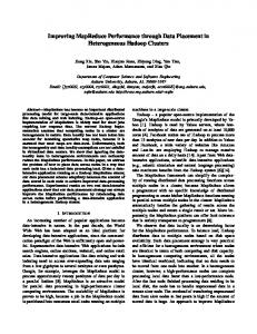
A MapReduce workflow involves a mapper and a reducer function. The way the mapper works is, every value has a key paired with it. The key uniquely identifies related values. The mapper and reducer functions always receive a pair of key and value. The output of both of these functions is always similar in the sense that they always return a key and a value. The difference between the mapper and reducer function is as follows: the mapper function will always return a single key and value for each key and value inputs. While, the reducer function will always return a single value for a list of values input for the same key. WordCount is a good example to understand how MapReduce works. The goal of WordCount is to count the number of times a word appears in a document. Here we utilize MapReduce to split up the document to the various mapper tasks, where each mapper task will emit a list of words and their counts for that part of the document. These lists are then sent to the reducer task to get an aggregate of all the mappers and produce a summary of the word and its frequency.
2.2
MapReduce Dataflow
The MapReduce Dataflow contains the following key components: an input reader, a map function, a partition function, a compare function, a reducer function and an
6
Figure 2.1: The Process of WordCount [1] output writer function.
2.2.1
Input reader
The purpose of the input reader is to split up the input into even sized chunks. The framework will then assign these split up chunks to the appropriate Map functions. The reader normally reads data from the storage subsystem and generates key value pairs, which are required by the mapper functions.
2.2.2
Map function
The map function will take the input generated by the input reader, which would be in the form of key value pairs and output a set of key value pairs.
2.2.3
Partition function
A partition function of an application will assign the output of the mapper function to the reducer. Using the modulo technique, the key is hashed to the number of reducers.
2.2.4
Comparison function
The comparison function is used to sort the input prior to delivering it to the reducer function.
7
2.2.5
Reduce function
The reducer function is called for each unique value in the sorted list provided by the comparison function. The reducer can iterate through the input and associate it with a key and output of zero or more values.
2.3
Apache Hadoop
Hadoop [1] is an open source framework for running applications on large clusters made up of commodity hardware from Apache. Hadoop utilizes the map and reduce functions, where the application is divided into several small fragments of work where each can be scheduled on any node in the cluster. The HDFS file system, which is a part of Hadoop, is used to store large amounts of data across all the nodes in the cluster. This allows the cluster to achieve a locality of data and use the maximum bandwidth of the cluster. The framework additionally manages failure scenarios.
2.3.1
HDFS
HDFS is optimized for storing huge files. These files can be streamed for use to the various map reduce programs which runs in the framework. HDFS utilizes clusters on commodity hardware and is the base of Hadoop MapReduce computation. It is created with the intention to carry on working in the face of failure without interruption to the user. HDFS Concepts: Blocks The HDFS blocks are optimized for large-scale data storage and retrieval. These blocks are much larger than the typical file system blocks. By default, Hadoop configures blocks to be 64MB in size. A block is a basic unit of a mapper functions input. HDFS Concepts: Namenodes and Datanodes A HDFS cluster works in the master slave pattern. A namenode is the master and the datanodes are the slaves. The namenode manages the file systems namespace and maintains all the metadata for all the files and directories, which are copied on to
8 the HDFS file system. The metadata information used by the namenode is stored as two files on the local disk. They are named the namespace image and the edit log. The namenode also knows exactly which datanodes the blocks of a file are located on. However, this information is not persisted since this information is reconstructed when the system starts. A software client accesses the file system by communicating with the namenode and the datanodes. The HDFS file system is mostly POSIX-like so the user can use normal file system utilities without having particular knowledge about the namenode or datanodes. The namenode is a very critical part of the HDFS file system. Without the name node, the file system is unusable. If the namenode crashes due to hardware failures, all the data in the datanodes will be lost, since the important metadata to construct the data from the datanodes would have been destroyed. Hence, it is critical that the namenode is resilient to failures. Hadoop provides two ways to make the namenode resilient: the first way is to back up the files that contain the persistent state of the filesystem metadata. The second way is that Hadoop can be configured so that the persistent state can be written in an atomic and synchronous way to multiple filesystems. Parallel Copying with DistCP DistCP is a program that comes with Hadoop, which is used to copy large amounts of data to and from the HDFS file system. This program is usually used to transfer data between two HDFS clusters. The program is implemented as a map reduce job where the task of copying is done by the mapper function that can run parallel across the cluster. There are no reducers involved in the process. The program tries to evenly divide the amount of work to the mapper functions by bucketing the files into roughly equal sized units. The way the number of maps is decided is in the following manner: each map will have a minimum of 256 MB of data to transfer. As an example, assume that 1GB of file will be provided four map tasks to carry out the transfer. When the data size grows very big, it is necessary that number of map tasks created to handle this data is limited to help maintain good bandwidth and cluster utilization. The DistCP command usage is hadoop distcp hdfs://namenode0/file1 hdfs://namenode1/file2
9
2.3.2
Hadoops Implementation of MapReduce
Task Assignment A job in Hadoop is split up into multiple tasks. Each of the tasks periodically communicates with the jobtracker to inform it whether its alive. This is called the heartbeat. The tasktracker also informs the jobtracker if it has completed its existing task and is willing to accept new tasks. Before the jobtracker can allocate a new task to the tasktracker, it will need to select a job from a list. Once the job is selected, the jobtracker will now split that job into multiple tasks and then assign the task to the tasktracker. Tasktrackers normally have a fixed number of slots for the mapper and reduce functions. This would mean that each tasktracker could run two mapper and two reducer tasks at the same time. Before the reduced task slots, the scheduler fills the empty map slots. So if the tasktracker has at least one map slot empty, the job tracker will select a map task or it will select a reduced task. For the scheduler to choose a reducer function it just looks up the next in the list of yet to be run reduce tasks. When it comes to the map task, it considers the network location of the task tracker and selects a task whose input split matches or nearly matches the tasktracker so as to keep the data local. Fault-tolerance Hardware and software failures are a part of reality. One of the major advantages of using the Hadoop framework is its ability to manage hardware and software failures. Task Failure A task can fail when the user code running the task for either a mapper or a reducer throws a runtime exception. When this happens, the JVM throws an error back to the task tracker and this is logged in the user logs. The task tracker then marks this task as a failure and is ready to run another task in this slot. Another possible type of error could be that the JVM of the task crashes due to a JVM bug, which could be caused by an environment issue. In this case too, the tasktracker will mark this task as failed and will request a new task. Task which hang are handled differently compared to the above cases. The tasktracker noticed that no progress has been made by the task for a long time and proceed to mark the task as failed and kills the hanging JVM. The framework can set a timeout for a task after which it will be marked as failed automatically.
10 When the job tracker is notified that a task has failed, it will reschedule the execution of the task. It will try and avoid rescheduling the task on a tasktracker where it previously had failed. If the same task now fails more than four times on different task trackers, then the entire job is marked as failed. For certain type of applications, a threshold can be set to the number of failures that are permitted. These are controlled by two values: mapred.map.max.attempts property for map tasks, and mapred.reduce.max.attempts for reduce tasks. There is a difference between a task being killed from a task failing. A task could be killed because the framework could decide that the task was a duplicate. Or it could be because, the tasktracker was running on failed or the job tracker marked all the task attempts running on it as killed. Users may also kill a failed task attempt through the web UI. Tasktracker Failure A tasktracker failure is detected by the failure to receive heartbeats by the jobtracker. The tasktracker could fail either by crashing, or running really slowly. In this case, the jobtracker would detect that the tasktracker is behaving erratically and could remove it from its pool of tasktrackers to schedule tasks on. Once the tasktracker has been removed, all pending tasks that were assigned to the tasktracker will now be rescheduled on to different task trackers. If a tasktracker reports multiple task failures over a period of time, its possible that the job tracker can blacklist the task tracker. The admin can then remove the blacklisted tasktracker from the cluster. Jobtracker Failure The only single point of failure in the Hadoop framework is the failure of a jobtracker. This failure mode has a low chance of occurring, since it would require the machine to fail. Task Scheduling Hadoop comes inbuilt with a choice of task schedulers. The default scheduler being the FIFO scheduler and there is also a multi-user scheduler called fair scheduler. The FIFO scheduler uses a very simple approach user jobs. All jobs from all users are put into a single queue. The framework takes the first job from the queue and runs it across the entire cluster. This is suboptimal in a multiuser environment since only one user’s job can be run on the cluster at a time. To overcome these shortcomings, the fair
11 scheduler was introduced. The fair scheduler aims to give every user an equal share of the capacity of the cluster. The fair scheduler shows progress on multiple jobs, which have been assigned to run on the cluster. For example, a short job belonging to one user will complete in reasonable amount of time, even when a long job of another user is running simultaneously. It is also possible to define custom pools with guaranteed minimum capacity defined in terms of maps and reduce slots, where weights can be set on these pools. The fair scheduler supports preemption which means that if a pool has not garnered its fair share for a certain amount of time, then the scheduler will kill tasks in pools running over capacity in order to provide the slots to the pool running under capacity a chance. Shuffle and Sort
Figure 2.2: The Process of Shuffle, Hadoop: The Definitive Guide [2] p 163 From the map output to the reducer input, the system performs a sort. This entire process is called the shuffle. The diagram [?] depicts how the shuffle works. The understanding of this process is important in order to optimize the map reduce program written by the user. The shuffle is a central concept to the map reduce framework. A circular memory buffer is allocated to each map task. This buffer is used by the map task to write out the partial reserves as they are being generated. When a threshold size is reached in the buffer (approx. 80%) a background thread starts to write the data to the local disk. Simultaneously, the map task could be refilling the circular buffer while the thread writes data to the local hard drive. The thread, prior
12 to writing out data to disk, will split the circular buffer into chunks, which will be sent to different reducers. Once the chunks have been decided, before writing the data to disk, they are sorted and then written to disk. If a combiner function has been specified, then the combiner is run before the output file is written. Compressing the map output as it is written to disc makes the write to disk faster, and saves disk space and reduces amount of data that needs to be transferred to the reducer. It is over HTTP that the output files partitions are made available to the reducers. The task tracker.http.threads property controls the number of worker threads used to serve the file partitions. For large clusters running large jobs, the default of 40 can be increased. On the reduce function, the map output file that is sitting on the local disk of the tasktracker (which earlier ran the map task) is now needed by the tasktracker that is about to run the reduce task for the partition. This is because the map output is required for its particular partition from several map tasks across the cluster. The reduce task starts copying their outputs as soon as each is completed - a process also known as the copy phase of the reduce task. In order to fetch map outputs in parallel, the reduce task has a small number of copier threads. By changing the mapred.reduce.parallel.copies property, once can change the default setting of five threads. When the memory buffer reaches a maximum threshold or reaches a maximum number of map outputs it is merged and written to disk. A background thread merges copies into larger, sorted files. After all the map outputs have been copied, the reduce task proceeds into the sort phase (also called the merge phase), which merges the map outputs, maintaining their sort ordering. This is conducted in a series of rounds. For example, there would be 5 rounds if there were 50 map outputs, and the merge factor was 10. At the end there would be five intermediate files and instead of a final round that merges these five files into a single sorted file, the merge directly feeds the reduce function. This is the reduce phase or the final phase, where the merge can result from a combination of in-memory and on-disk segments. The reduce function is instantiated for each key in the output which appears in a sorted order. The output is written directly to the output file system or HDFS.
13 Speculative Execution The goal of the MapReduce model is to split jobs into multiple tasks and execute them in parallel. In theory, this should significantly reduce the processing time of the job, as compared to if it were run sequentially. However, the drawback here is that if a single task is delayed it causes the entire job to take a longer time to complete. For large jobs, the possibility of a single task getting delayed is very likely. The reasons that could delay a single task are: hardware malfunctions, software bugs, configurations, etc. These reasons could be difficult to detect since most jobs complete successfully - but they take a longer time. Hadoop does not try to detect slow running tasks. When the framework detects a slow running task, it will spawn a duplicate task to do the same function as this task. This is known as speculative execution of tasks. It is vital to understand that this duplicate or backup task is never started at the same time than the task it is meant to shadow. This begins only when the framework detects that the original task is taking longer than normal. When the original task has been completed, any duplicate task that exists will naturally be killed, and vice versa. The speculative execution task can be controlled via configuration parameters.
2.4 2.4.1
Typical MapReduce Applications WordCount
In order to measure the frequency of a single word in any given input data, the WordCount application is used. When the size of the input is large enough, we receive greater benefit by having a local combiner since the data is much more aggregated after the combine.
2.4.2
InvertedIndex
The InvertedIndex is a data structure, which is used for indexing documents. It does it by storing a mapping of the contents to its location. It enables fast full text searches and also supports incremental index building. The two popular forms of inverted index are record inverted index and word inverted index, where the record inverted index contains
14 a list of references to each word. The word inverted index contains the position of the word within the document. In the map reduce paradigm, the map function will parse the input document and spit out a list of word and IDs (document IDs). The reduce function accepts all these inputs from the mappers and emits a word and a list of document id pairs. This output is basically the inverted index.
2.4.3
Sessionization
In order to determine user behavior analysis, web logs of online user activity are an important data for web companies. In this case, each user click on web pages are aggregated to produce large amounts of data. Often, the first task is to identify a visitor session [3]. Within web data analysis, sessionization is good example of the mapper reduce function. A log data of user clicks is divided according to sessions or the total number of clicks that take place within a particular span of time. Important click patterns can be detected from such methods, and is usually used to monitor fraud detection, revenue prediction, ad promotion, etc. For example, within the same session, one can sessionize two clicks of the user that occurs within thirty minutes C assuming that the second click follows from the first click. On the other hand a new click after the previous one, is considered irrelevant and as is treated as a new session. Example of web click (web page visitor mouse activity) schema and data as follows: Create Table WebClicks (IP varchar(16), ClickTimestamp timestamp, URL varchar(200)) 153.65.20.33 2008-02-03 14:33:15 ebay.com 153.65.20.33 2008-02-03 14:44:15 dvd.shop.ebay.com 153.65.20.33 2008-02-03 14:59:08 netflix.com 153.65.9.89 2008-02-04 11:02:19 amazon.com 153.65.9.89 2008-02-04 11:33:04 amazon.com/travel 153.65.9.89 2008-02-04 11:48:27 travelocity.com If 30 minutes is the user specified period for identifying the same visitor session. After running the sessionization task, the output should be as follows: 1 153.65.20.33 2008-02-03 14:33:15 ebay.com 1 153.65.20.33 2008-02-03 14:44:15 dvd.shop.ebay.com/
15 1 153.65.20.33 2008-02-03 14:59:08 netflix.com 1 153.65.9.89 2008-02-04 11:02:19 amazon.com 2 153.65.9.89 2008-02-04 11:33:04 amazon.com/travel 2 153.65.9.89 2008-02-04 11:48:27 travelocity.com Since each new click is within 30 minutes of the previous click, the 3 clicks from IP 153.65.20.33 receives the same session number. However, for IP 153.65.9.89, the second click (2008-02-04 11:33:04) gets a new session number because it is more than 30 minutes after the first click.
2.5
Related Work
Traditionally, the MapReduce [4]programming paradigm assumed the operating cluster was composed of tightly-coupled homogeneous compute resources that are generally reliable. Previous work has shown that if this assumption is broken, that MapReduce/Hadoop performance suffers. LATE [5]was the first work to point out and address the shortcomings of MapReduce in heterogeneous environments. They specifically focus on the observation that under computational heterogeneity, the mechanisms built in to MapReduce frameworks for identifying and managing straggler tasks break down, and propose better techniques for identifying, prioritizing, and scheduling backup copies for slow tasks. In our work, we assume that nodes can be heterogeneous since they belong to different data centers or locales. Techniques to improve the accuracy of progress estimation for tasks in MapReduce were reported in [6]. Tarazu [7] demonstrate that despite straggler optimizations, the performance of MapReduce frameworks on clusters with computational heterogeneity remains poor as the load balancing used in MapReduce causes excessive and bursty network communication, plus the heterogeneity amplifies the Reduces load imbalance. They address the problem with communication aware balancing mechanism and predictive reduce load-balancing. Mantri [8] explores various causes of outlier tasks in further depth, and develops cause- and resource-aware techniques to act on outliers more intelligently, and earlier in their lifetime. Such improvements are complementary to our techniques. The work above mainly focus on computational heterogeneity with in one single cluster, However, the loosely-coupled and network-heterogeneous nature of the systems we address adds an additional bandwidth
16 constraint problem, along with the problem of having widely-dispersed data sources. MOON [9] explored MapReduce performance in volatile, volunteer computing environments and extended Hadoop to provide improved performance under situations where slave nodes are unreliable. In our work, we do not focus on solving reliability issues; instead we are concerned with performance issues of allocating compute resources to MapReduce clusters and relocating source data. Moreover, MOON does not consider WAN, which is a main concern in this paper. Work in wide-area data transfer and dissemination includes GridFTP [10] and BitTorrent [11]. GridFTP is a protocol for high-performance data transfer over highbandwidth wide-area networks. Such middleware would further complement our work by reducing data transfer costs in our architectures and would further optimize MapReduce performance. BitTorrent is a peer-to-peer file sharing protocol for wide-area distributed systems. Both of these could act as middleware services in our high-level architectures to make wide-area data more accessible to wide-area compute resources. Other work has focused on fine-tuning MapReduce parameters or offering scheduling optimizations to provide better performance. Sandholm et. al. [12] present a dynamic priorities system for improved MapReduce run-times in the context of multiple jobs. Our work is concerned with optimizing single jobs relative to data source and compute resource locations. Work by Shivnath [13] provided algorithms for automatically finetuning MapReduce parameters to optimize job performance. This is complimentary to our work, since these same strategies could be applied in our system after we determine the best MapReduce architecture, in each of our respective MapReduce clusters. Several works in SIGMETRICS [14] [15] has presented the idea of addressing similar problems as this paper. However, these works are not providing an end-to-end overall improvement of the MapReduce dataflow.
[14]optimize the reduce data placement
according to map’s output location, which might still end up trapping data in nodes with slow outward links. [15] has presented similar idea of shuffle-aware scheduling, but not considering the scenario that data sources are widely distributed and not co-located with computation clusters. The ICMR algorithm provided in that paper can make use of our mechanisms to improve the performance of MapReduce under such environments. Starfish [16] proposed a self-tuning architecture which monitor the runtime performance of MapReduce system and tune the Hadoop parameters accordingly. However,
17 the approach they take to realize performance optimization is by tuning the Hadoop configuration parameters, in our approach, we are focusing on mechanisms that directly changes task and data placement. Their work could be complementary to ours helping tuning the cluster. Pipelining MapReduce has been used in MapReduce Online [17] to modify the Hadoop workflow for improved responsiveness and performance. But they assume input data is located with the computation resource and didn’t address the issue of pipelining push & map.This would be a complimentary optimization to our techniques since they are concerned with the packaging and moving of intermediate data without storing it to disk in order to speed up computation time. Our mechanism could be used as a guidance of data distribution.
Chapter 3
Hadoop’s Performance under Distributed Environment 3.1
Experiment Scenario
Here we propose a typical scenario of MapReduce when data and computation resources are both widely distributed. The computation resources are located at different locations of the world and thus have obvious delay when transferring data between source and computation clusters or between computation clusters. In PlanetLab we used a total of 8 nodes in two widely-separated clusters C 4 nodes in the US, 4 nodes in Europe. In addition, we used one node in both clusters as our data sources. For each cluster, we chose tightly-coupled machines with high internode bandwidth (i.e., they were either co-located at the same site or share some network infrastructure). In the presence of bandwidth limitations in PlanetLab and workload interference with other slices, the intersite bandwidth we experienced was between 1.5C2.5 MB/s. On the other hand, the inter-continental bandwidth between any pair of nodes (between US and EU) is relatively low, around 300C500 KB/s. The exact con?guration is shown in Tables 1 and 2. Due to the limited compute resources available to our slice at each node, we were limited to a relatively small input data size for our experiments to ?nish in a timely manner, and also to not cause an overload. At each of the two data sources, we placed 400 MB plain-text data (English text from some random Internet articles) and 125 MB random binary data generated by RandomWriter in Hadoop. In 18
19 total, there was 800 MB plain-text data and 250 MB random binary data used in our PlanetLab experiments. The number of Map tasks by default is the number of input data blocks. However, since we were using a relatively small input data size, the default block size of 64 MB would result in a highly coarse-grained load for distribution across our cluster. Therefore we set the number of Map tasks to 12 for the 250 MB data set (split size approximately 20.8 MB).
3.2
Experiments Result and our Observation
Figure 3.1: Figure 3: Architectural approaches for constructing MapReduce clusters to process highly-distributed data. This example assumes there are two widely-separated data centers (US and EU) but tightly-coupled nodes inside the respective data centers. We have proposed 3 different architectures of MapReduce job execution(Figure??). Global MapReduce (GMR), which is simply running Hadoop over all of our machines, push all the data to HDFS via HDFS-put or DistCP and then run the MapReduce job on all the machines, is one of the typical way of using Hadoop in most of current industry usage. HDFS-put is the API provided by Hadoop to import data into HDFS, which is directly copying data from data source to several HDFS nodes specified by the master, which is used to import data into HDFS. DistCP is a widely used Hadoop API for copying data from one HDFS to another HDFS, it will start a MapReduce job to copy in parallel. Besides GMR, we introduced two other different architectures: Local MapReduce(LMR)
20 and Distributed MapReduce(DMR). In LMR, we first push all the input data to one of the data centers and do the computation with only machines in that data center locally. In DMR, we run two separate MapReduce jobs in each data center with only those local input data, and we combine the result in the last step. The Figure 3.1 shows the three architecture and the performance is illustrated in Figure 3.2,3.3.. From the result, we think the following observation is interesting:
Figure 3.2: Performance of Different Architectures First, importing remote data is time consuming. In the case of LMR and GMR, the time taken by the push phase has taken up a considerable fraction of overall running time of the job, and this is mainly because of the network delay in the wide area network. This shows the potential of benefitting from speeding up the push-map process. Secondly, Hadoop’s decision of data and task placement is not optimizing the overall execution time on a global view. For the shuffle-light jobs, as shown in Figure??-(a) there is not too much difference in MapReduce computation time. For the shuffle-heavy jobs, the three different architecture showed quite different performance in the three phases after push phase. As we can see in Figure??-(b). In LMR, by manually forcing the data to be transferred to one single cluster before map
21
Figure 3.3: Performance of Different Architectures computation and data ballooning, we can see the time taken by shuffle, reduce and result combine is greatly reduced and it is much less than that of GMR and DMR. This shows that a data and task placement made with a global view can potentially reduce the computation time by transferring less data along slow links.
3.3
Problem Definition and Challenges
Here we recognize the problem as a optimization problem that we are trying to improve the efficiency of dataflow as well as the use of computation resources. And this problem contains two subproblems: • For a single remote data source and single computation cluster, How to efficiently import the data to computation clusters? As the data source doesn’t have good network connections to the computation resource, and the import is an unavoidable process for computation to happen, thus we need to decrease the cost of this process in the overall computation time. • Task Scheduling in Distributed Environment Briefly mention that hadoop can do a good map-local optimization, but the decision could be a bad global decision when shuffle is heavy
22 Introduce our solution: shuffle-aware scheduling (it is also reduce-aware, but as the focus of the problem is mainly on shuffle, I am thinking of calling it like that) State that this is a lower-level task scheduling since it is focusing on task scheduling within a job, different from most of the previous work, mention works in the related area
Chapter 4
Improving Hadoop’s Mechanisms 4.1
Modification of Hadoop Mechanisms
Figure 4.1: System Architecture In order to solve the problem described in section 2, we designed and implemented our mechanism base on the 1.0 version of Hadoop system. Figure4.1 showed the highlevel system architecture. The dark-colored blocks represents the new modules we are adding to the original Hadoop system. Which are listed as following: • Pipelining Push&Map • Fine Grained Task Placement • Network Monitoring Module
23
24 For pipelining push & map, By making use of Hadoop’s mechanism to execute map task on remote data, we can start map computation on each node as soon as it has get the data from the data source. In this way we removed the global gap between push & map and can get some overlapping. In our mechanism that implemented based on this, we replicate each block to local cluster, then we execute local map task on the block. In this way, the input data can be completely imported after the map execution, and the re-execution of map task under failure is faster. For fine-grained task placement, As Hadoop’s task are all working in a pull-style to fetch the input data. We make use of this nature to bind data placement and task placement together and so they could both be controlled by task scheduler. We modified the API Hadoop has provided for implementing customized task scheduler to allow more control from the scheduler to decide which task to assign. The network monitoring module is used to collect the network info prior to job and during runtime. It includes monitoring module and a database that could be directly accessed by the task scheduler.
4.1.1
Pipeline Between Push and Map
As we have analysed in Section 2, under widely distributed environment, when the network connection from the data source to the computation resources is not as fast as inner-data-center networks, the time taken by merely importing data from the source to the computation cluster is non-trivial. The most typical way of doing computation on remote data with Hadoop is “push-then-map”, which firstly do an HDFS-put or run a DistCP job(or any other importing jobs) to import the data to the computation cluster, then start the MapReduce job. This certainly leaves a global gap between push and map phase, and a natural solution would be trying to remove the gap by pipelining this two phase and thus speed up the overall process. Hadoop Map Task’s Remote Execution Hadoop has provided mechanism to run map task directly on remote data, with Hadoop’s implementation, if the remote data is located on datanode of HDFS(could be a separate remote HDFS), the mapper can directly remotely open the file and read from remote HDFS, and all the serialization work is handled by Hadoop automatically. In this case,
25 in a single map task it is a sequential execution, it read in one line remotely and apply map function on it and read the next line. However, when there are multiple map tasks(which is often the case for MapReduce jobs), we can get some benefit from a coarse-grained pipelining: some of the map tasks are in their push phase while others have started map computation. This is better illustrated with Figure4.2 . In order to show the difference in performance, we ran WordCount on plain text data on our 3 node cluster, set the emulated network speed from the source to cluster limited as 4MB/s. We prefer WordCount as the map time takes up a large fraction of total running time. The result in Figure4.3 showed the difference in performance between push-then-map and pipelined push and map.
Figure 4.2: Overlap Example However, Hadoop’s remote execution is not widely used for most job execution on remote data, people still prefer the push-then-map approach in practice, as Hadoop’s remote execution has following problems: 1. With remote execution, the data is not actually ’imported’ to the computation cluster as mapper is directly running map functions on each piece of remotely read data, which is not convenient if we need to run some job on the same input in the future. 2. The remote execution is not well designed for fault-tolerance as there is no local replicas of each block and Hadoop will always go back to the remote source under task or node failure. Which will result in a poor performance when failure rate increases. Figure4.4 is an example of performance problem of remote execution under failure, in
26 which we ran the same experiment as above and manually introduced 1 wave of task failure at the last wave of map task.
Figure 4.3: Comparing Pipelining with DistCP
Figure 4.4: Overlapping Push and Map
Our Solution: Copy & Local Map We did some simple change to Hadoop’s remote map execution mechanism so solve the problem above while still preserving the pipelining benefit. In each map task, we firstly copy the whole block to local cluster and then run the map task locally. In detail, it works as following: 1. For each map task, upon getting the split, first check its location, if the split
27 locates on a remote host, then instead of start to read the file and execute map function at once, we firstly copy the whole block to local cluster as a HDFS file and thus it is replicated as ordinary file 2. then change the split location to that local file, start to execute the map function locally. This approach is called Copy and Local Map(CLM). Algorithm 1 CopyAndLocalMap CopyAndLocalMap ( S p l i t i n p u t S p l i t , F i l e S y s t e m l o c a l F i l e S y s t e m ) i f ( i n p u t S p l i t . l o c a t i o n != COMPUTATION CLUSTER HOSTNAME) Path p = REPLICA PATH+i n p u t S p l i t . s t a r t P o s i f ( ! localFileSystem . hasFile (p)) DFSCopy ( i n p u t S p l i t . l o c a t o n , p ) inputSplit . location = p ExecuteMap ( i n p u t S p l i t )
With our approach, the overlapping is preserved so the performance is almost the same as Hadoop’s remote map execution; and as the split location is pointed to a local file, it has the same recover time as local execution under failure; input file is imported and replicated; and this makes the speculative execution faster. Figure4.5 shows the performance under emulated environment. We ran WordCount on 1G plain text data on our 6 node cluster, set the emulated network speed from the source to cluster limited as 4MB/s. To test the performance under failure, we ran the same experiment while manually introducing 3 task failure to the last wave of map task(Figurefig:Failure-CLMRM-PTM). As the re-execution performance of map task in CLM is the same as local execution, CLM out-perform RemoteMap when failures are introduced. And we can expect even more benefit over RemoteMap if the failure rate of map task increase. One problem we left over is that we didn’t try to build a more fine-grained pipeline by overlapping the push and map within each map task, we can implement this feature by keep reading and buffering the whole block and let map function take its input from the buffer. There are basically two reasons we didn’t prefer to finish this: Firstly, this will increase the memory burden, especially when there are multiple map slots on one single mapper. A possible case is that some map task is using a big fraction of memory to sort the output while several other map tasks are buffering a lot of data in the memory. We may handle this problem with a well-controlled memory
28 management but that would introduce more complexity. Secondly, fault-tolerance will be more complex. If we start the map task before we completely have the input block located in the computation cluster, when failure happen ( most of time during map task execution), we don’t have the complete block locate in the computation cluster by that time. This will bring up problems like when to checkpoint the buffered data during map task execution, and how to synchronize among all the node as re-execution or speculative execution might be scheduled on some other node. In general, this approach might introduce more risk and complexity into the current system, so we prefer to leave it as a future work to figure out how much benefit we can get from this fine-grained pipelining and how can we handle the memory usage problem and the fault-tolerance problem.
Figure 4.5: Performance of CLM
4.1.2
Mechanisms for Task Placement Control
Another problem we are observing in Chapter 2 is that with network and computation heterogeneity, where does the data flow during the whole MapReduce process has a non-trivial effect on overall performance. An intelligently controlled data placement can prevent a lot of unnecessary data transferring over slow network and thus result in a shorter execution time. In order to achieve a optimized data and task placement, we need mechanisms that could allow a full control over dataflow and task scheduling.
29
Figure 4.6: Performance under failure However, Hadoop’s current mechanisms doesn’t give user enough freedom to control them. This section will introduce how we address this issue.
4.1.3
Control Dataflow With Task Placement Control
Hadoop’s task execution mechanism is actually binding data placement with task locations. All the task execution is working in a pull-style. For map task, if the input data is non-local, then the mapper will pull data from the remote location and run map function on the data. In our scenario that have distributed data sources, we can control the fraction of data sending from each data source to each mapper by intentionally assigning map tasks. For reduce task, each reducer will fetch intermediate output from all mappers. Assuming the user-defined hash function can achieve even distribution of keys to all reduce partitions, then fraction of data processed by each reducer can also be controlled by changing the number or size of reduce tasks on a certain node. Thus, as long as we could have control over the size of input data and the placement of each task, we can control the overall “sources-mappers-reducers” dataflow. Figure4.7 illustrated the basic idea of dataflow control with task scheduling. We can achieve a more intelligent decision by implementing a more smart task scheduler. However, the interface that Hadoop has provided for task scheduler is intended for Job-level task scheduling, which only trying to decide whether a task tracker could get a task or not, it doesn’t provide the interface to choose some specific tasks to be assigned to a tasktracker. Therefore, in order to provide the mechanism of data-flow controlling,
30
Figure 4.7: Dataflow Control with Task Placement our work is based on changing the API that Hadoop provided for task schedulers to enable fine-grained task scheduling. Map Task Placement Control Hadoop has provided a simple API for task scheduler to get some map task for a certain task tracker. And this API has some intelligence of data locality if the user has provided some data location info. However, this doesn’t allow a fine-gained control over specifically which task to assign to which node and thus cannot make full use of the info that task scheduler may have. In our approach, we have extended that API to take a set of task input split location that the node could pull data from. And the task scheduler will use this set of locations as a filter when searching for task candidates. The set of location could be either actual nodes or racks. The task input split locations to be put in the set are decided by the actual scheduling algorithm used in the task scheduler. In this case, the data locality feature that originally provided by Hadoop is still preserved. With this approach, user could have a fine-grained control with job-level task scheduler with some minor change. Figure4.8 illustrated how this works.
31
Figure 4.8: Map Task Placement Control Reduce Task Placement Control The main target of reduce task scheduling is to control the fraction of data that is processed by each reducer. Hadoop has provided API that could get a random reduce task from the unprocessed queue and assign it to a certain tasktracker. Base on Hadoop’s mechanism, we have two different choices to implement the mechanism that could control the size of data got processed by each reducer: 1. Create reduce tasks with different partition size (different range of keys) and assign a specific reduce task to a specific tasktracker. We call this single-wave, different partition size(SWDS) approach since we only try to create as many reduce tasks as the available reducers, so all the reduce tasks should be processed in one-wave. 2. Divide the whole intermediate data into smaller pieces by having more reduce tasks, assign different number of reduce tasks to each tasktracker. We call this multiwave, different number of reduce task(MWDN) approach since in this approach, we tend to create more reduce task than available reducers so that we can have more freedom to assign different number of reduce tasks to each reducer, in this case, some of the reduce task will have to wait till there are reduce slot available. The main idea to implement SWDS is: Assuming user has provided a hash function that could result in even distribution of data, then by creating a customized partitioner, we can generate partitions with different sizes and thus the data distribution of reduce tasks is unbalanced. Then by modifying Hadoop’s API of getting reduce task to assign, we can assign a reduce task with certain partition number to a certain tasktracker. Thus
32 we can create a controlled data distribution of reduce task by maintaining a mapping from tasktracker’s name to partition numbers. Having multiple waves of reduce task is basically making use of the mechanism that Hadoop has originally provided. We just need to decide the number of reduce task base on the granularity we want to schedule the reduce tasks. Then we just need to maintain a mapping between tasktracker and the number of reduce tasks in the task scheduler and stop assigning task to a certain node if there is no more reduce task need to be assigned to it. We have listed the advantage and disadvantage of the two approaches in Figure4.9.
Figure 4.9: Advantage and disadvantage of the two reduce control approaches
Sensitivity Analysis of Number of Reduce Tasks As there are several factors affecting the overall performance under different environments. We try to compare their performance by isolating different factors with 4 questions and we will answer these questions with experiments. In our experiments, we are more interested in the case when the job is shuffle-heavy (or reduce-heavy) because that would show more benefit of reduce controlling mechanism. And we don’t expect to improve Hadoop much under shuffle-light cases. For experimental usage, we created a synthetic job which could generate a workload with controllable map, shuffle and reduce heaviness. We did this by casting controlled amount of data in mapper and reducer regardless what input is. We will use that in following experiments. We listed following questions trying to compare the two approach and see the insight of Hadoop’s reduce task mechanism.
33 1. When there is no overlap between Map and Shuffle, is having multiple waves of reduce task beneficial or harmful to reduce performance? 2. Is overlapping Map and Shuffle always beneficial? Is there any cost brought by having more overlapping? 3. Under which condition should we choose which approach? 4. Can we combine these two approach? For question 1, It is widely acknowledged as a rule of thumb that we should have less reduce waves. And the common explanation is that it will allow more overlap between map and shuffle. However, when there is no overlap at all, is that always a bad decision to have more reduce task? Especially when shuffle is heavy? In this experiment, we setup 4 nodes, using 2 as mappers and the other as reducers. We give each reducer 2 reduce slots. When there are multiple reduce tasks, we set the wave to be 5. The synthetic job is set to have a 2x data ballooning after map processing to make the job shuffle-heavy. We avoid the overlap between Map and Shuffle by setting the reduce late start factor to be 1. In this case, any reducer won’t start to pull data from any mapper until the last mapper is done. Interestingly, the overall reduce time decreased when there is multiple wave of reduce tasks(Figure4.10), despite the well-known fact that more reduce task will introduce more overhead. After examining the data reading time of each reduce task, we found that the time taken by reducer to read the merged input is longer when there is less waves of reduce task. And this difference is because when there is more reduce task, each task is smaller, which makes it easier to fit in memory for direct reading and thus avoid the overhead of disk I/O. The difference is smaller when we increase the memory that could be used for reducer’s buffer. Thus, we can see if the intermediate data is large enough and it cannot fit in memory, using more reduce task can get some benefit by avoiding more disk I/O. However, it is not always better to have more reduce waves, if the reduce task is already small enough to fit in memory, then further increasing the number of reduce task will only increase pure overhead. Figure4.11 showed a trend of have 1-10 waves of reduce tasks.
34
Figure 4.10: Relationship between reduce time and number of reduce waves
Figure 4.11: Reduce time of one-wave as multi-waves For question 2,It seems intuitive that if we overlap two sequential process, we should always get some improvement in performance. Just as overlapping push and map. However, one important fact is that mapper is still doing computations or writing to harddisk while reducer is pulling data from it. The pulling process might interfere with the ongoing work on the mapper, and there are potentially network congestion brought by shuffle and remote map competing for network resources. We set our experiment on the same cluster as above. We allow the overlap by setting the late start of reducer to be 0.2. So the reducer will start to pull data when 20% of map task has completed. The other setup is the same as above. As shown in Figure4.12, the map execution time gets longer when there is more
35 overlap between map and shuffle. This brings down the benefit we get from overlapping map and shuffle. And with the advantage of having multiple reduce waves as we mentioned in (1), in terms of overall execution time, multiple waves beats single wave. Thus, when shuffle is heavy, the cost introduced by reading heavily from a busy mapper and the network contention of shuffle and remote map might be non-trivial and it might reduce the benefit we get from overlapping. In general, when the job is shuffle heavy, overlapping map and shuffle might not actually bring so much benefit as it seems.
Figure 4.12: Performance Between Single Wave and Multiple Wave of Reduce Task For question 3,In terms of choosing between the two approaches, with the analysis above, we can see the decision depends on the job’s nature and the cluster’s condition. If all the node have large enough memory to fit large reduce inputs, then we can choose larger task to get more overlap. Also, if the mapper is powerful enough, it might not be affected by the heavy reading from reducers. Above all, if the job is shuffle-light, as examined by numerous developers and researchers, have less reduce waves and getting more overlap is still more beneficial. In our experiments in section 7, we prefer to use the MWDN approach, as most of our experiments are shuffle-heavy and it is simpler to use. But we set the same number
36 of reduce tasks for any control group to maintain the fairness of comparison. For question 4, we can combine them as different number of reduce task in difference size(DNDS) approach. In this case, we assign different number of reduce tasks to difference nodes and the size of the tasks varies. And this is combining the advantages of both approaches. For powerful node with good network and enough memory, we can assign one single reduce task to it so it can benefit from having more overlap; For smaller nodes, we can assign multiple waves of smaller tasks to these node to fit in memory and allow more dynamics. We did one experiment on EC2 as an example of benefit we can get from this approach(Figure4.13). We use 1 single medium instance(4GB memory) and 4 micro instances(613MB memory). In this experiment, we assign 50% of reduce data in one large reduce task to the medium instance, and the rest in 10 small reduce tasks. The networks are all 16M/s inner network, thus avoided complexity in network heterogeneity. The ballooning factor is set to be 2x. Notice that the ’reduce time’ in Figure4.13 is the time taken by reduce after Map is 100% complete, thus with more overlap, the ’reduce time’ is shorter, but the actual reduce running time could be much longer. However, it is not always easy to make decisions on how large a task should be and how many task we should assign when using DNDS. Since it depends on factors like memory available on each node, network condition among nodes, failure rate, and the overall job nature. So far we don’t have any well-defined method that could make this decision intelligently, and we will leave the research about DNDS as future work.
Figure 4.13: Different Number Different Reduce Task Size
37 In Figure4.14 we showed the performance of the MWDN and SWDS comparing with the baseline by running synthetic job in the same setting as in Q1,Q2. The baseline is having only one wave of reduce task and the workload is evenly distributed. In the case of using the two approaches, we manually compute a optimized reduce data distribution as input.
Figure 4.14: Performance of Reduce Control
Chapter 5
Shuffle-aware Scheduling use of these mechanism to achieve a better performance than original Hadoop. And we are providing two different task scheduling algorithms and we will compare its performance with Hadoop’s default task scheduling’s performance under simulated environment in this chapter. Here we are trying to show that with the approach above, it is possible to plug-in some static distribution or some simple heuristic to improve the performance of Hadoop under distributed environments. And these mechanisms could be a support to any future endeavors that trying to improve Hadoop’s performance with task scheduling approaches.
5.0.4
Hadoop’s Default Task Scheduling
As we are using Hadoop’s default task scheduling as the baseline, in order to make a fair comparison to it, we firstly need to understand how Hadoop’s default task scheduling works and what are its advantages and disadvantages. There are three important aspects we need to know about Hadoop’s default task scheduling:(1) Need-based greedy approach (2) Data-locality and (3) Speculative Execution. (1) Need-based greedy approach Without any external info about the network topology or data location, Hadoop by default will always try to make full use of the cluster, which is a simple need-based approach: Whenever a tasktracker is idle, it will ask for task from the jobtracker, as long as the task queue is not empty and the tasktracker is ’able to handle the task’( task
38
39 that we have chosen haven’t fail on that tasktracker, the tasktracker still have enough disk space and memory, etc.), the jobtracker will assign a new task from the queue to that tasktracker. In this way, if a tasktracker is fast in completing tasks, it will get more task to do. (2) Data-locality Even under widely distributed environments where moving data around might be costly, Hadoop can do a good job on map task scheduling with data-locality feature. This feature requires user to provide some ’data locality’ info to the jobtracker by setting the task input split location as ’where it is supposed to be most local’. With this information, as described in Chapter 4.1, the map task runner will try to fetch the input data from where the split location has indicated. With this feature, when there are multiple copy of input data, the tasktracker will always start form the ’most local’ one. Another import part of this feature is the locality wait, which introduced by [18] and is widely used in popular schedulers like Fair Scheduler. Locality wait is also based on a simple idea that instead of assign the task right away to some tasktracker that is idle but far away from the data source, it might be a better choice to wait for a while and assign the task to a more local tasktracker. According to [18]. the locality wait can almost guarantee data locality during map phase. (3) Speculative Execution The task scheduler’s decision might not always be a good decision for all the time. The speculative execution feature can be regard as a role that rescuing the cluster from previous wrong decisions. The general idea of speculative execution is simply trying to run a speculative copy of a task that is slow in progress. This copy is often scheduled to run on some idle tasktrackers, intuitively this will do no harm and can possibly achieve better performance. Base on the features listed above, we could see that Hadoop can do a good job for map task scheduling. However, this is not always a global optimal decision. According to what we have observed in Chapter 2, the LMR is basically an example that an artifact task scheduling outperform original Hadoop. The local-optimal decision made by Hadoop might be even conflicting with the global optimal decision. If map task’s location is decided, then the reducer must pull data from the same location, if the mapper appear to be a node with slow links to reducers and the size of intermediate
40 data that need to be shuffled is large, then the data transmission cost will be nontrivial. Figure5.1 is a case of getting data trapped in a fast mapper. Suppose all nodes are homogeneous, as the link from source to Node1 is fast, Node1 is tend to finish it map task faster and ask for more, finally result in data trapped in Node1 as it is very slow during shuffle. Interestingly, the speculative execution might also do harm in this case because the speculated task might finished earlier and the intermediate data end up trapped in a node that is a bad source to fetch data from.
Figure 5.1: Data getting trapped The most intuitive way to let the scheduler make a better global decision is to make it more aware of the phase afterwards, and make decision base on the estimation of the performance of the whole process, we call it Shuffle-Aware Scheduling. It is actually not only ’shuffle aware’, it means trying to make decision base on the estimation time of every phase of the MapReduce job (Push, Map, Shuffle, Reduce). We call it ’shuffleaware’ is because this is some awareness that Hadoop’s default scheduling doesn’t have, and it will show more obvious benefit when the job is shuffle heavy (like Inverted Index, etc.). Respectively, we call Hadoop’s default scheduling strategy Map-Aware Scheduling, which is only aware of information of map phase and only trying to optimize map phase.
5.0.5
Static Approach
The static approach is basically trying to make a static decision of optimal task scheduling base on some information we have collected from some sampling job and network monitoring before we actually start the job. This could be regard as the basic use case
41 of our mechanism, that is, if we have some already computed distribution we believe is optimal, we can use the mechanism to achieve that. Base on the mechanisms we have provided above, we just need to input the optimized task distribution we have computed as a static input to the task scheduler, and the task scheduler just schedule the task accordingly. In our approach, the tool we are using to compute the optimal distribution of task is a LP-solver which models MapReduce job as a Linear Programming problem [19], and the solution of the LP problem will be the distribution of data from each source to each mapper and the fraction of all intermediate data that is processed by each reducer. When applying the static approach, the speculative execution is often turned off as it might result in a different distribution from what we have computed, which may finally lead to a sub-optimal decision. The advantage of static approach is that it is making decision with more knowledge and is generally making a more optimized decision. The disadvantage is that it is time consuming to compute the optimal solution and thus we cannot afford to re-compute and change the distribution during runtime if the environment changes. In this case, a previously optimal global decision might turn out to be a sub-optimal decision or even a very bad decision.
5.0.6
Dynamic Approach: Estimated Map and Shuffle Algorithm
The intention of having a dynamic approach, or a simple heuristic, is because sometimes we may want the decision making process to be more light-weighted and doesn’t require a lot of knowledge, so that we can always make a decision with some extent of intelligence during runtime according to the change of environment. The heuristic doesn’t have to give an optimal decision as it doesn’t have as much information as the static approach. In our design, this algorithm is trying to avoid a bad global decision that result from attempting only to optimize one phase locally, on the other hand, it should still show some benefit over Hadoop’s Default approach. In general, this is another example of using our mechanisms to improve the data and task placement. The dynamic approach could show that the mechanisms we provide in section 5 is not only useful when we have a static optimized distribution as input, we may also use it to implement run-time decision making.
42 The dynamic approach we are providing is called Estimated Map and Shuffle Algorithm (EMS Algorithm). The basic idea behind EMS is to avoid two cases: 1. Avoid trapping data in mappers with slow outward link. 2. Avoid sending too much data to reducers that have very slow inward link When the cost of moving data during shuffle phase is high, we should be more careful when we allocate map tasks, because a good scheduling for map phase might result in data being trapped in some node that have slow out-going link. The task scheduler should be aware of possible shuffle time when making decisions during runtime. Another case we are trying to avoid here is that some node S with very slow links coming in from all the other node to this node. In this case, if we decide to send a lot of data to node S during shuffle phase, the shuffle phase for all node will be estimated as very slow as S could be the bottleneck. An alternative choice would be decide to send less data to S during reduce phase. In brief, the EMS algorithm works as follows: Firstly, compute the data distribution for reduce phase, we compute this base on network link and computation capacity, if we don’t have enough info, we assume an even distribution. Each reducer will get its computed distribution + reduce strictness(Rs), which is a user-defined value to control the strictness of how the scheduler assign task according to the pre-computed reduce distribution. During runtime, for every ¡data source, mapper¿ pair, we maintain an estimated map shuffle time(EMST) value, which is computed base on the network link speed, previous map computation time, size of intermediate data located on the mapper and the fraction of data to be shuffled to each reducer. We update EMST value as the job proceed, if the EMST of any ¡data source s, mapper m¿ pair is large enough to exceed slow allowance(Sa)+min(EMST), in which Sa is a threshold set by the user to control the aggressiveness of the algorithm, then the tasktracker will temporarily stop assigning map task from source s to the mapper m. Until the EMST of other node has increased as map output accumulate on these node to bring m’s EMST back to below Sa+min(EMST).
43 Estimated Map and Shuffle Time As mentioned above, the definition of EMST is: EMST = Estimated Time to Get Free Map Slot+Estimated Map Time+Estimated Shuffle Time In which the Estimated Map Time is based on the last map execution time from the same source; And the Estimated Shuffle Time =max( for each reducer R{ (Intermediate Data Size Located on that Mapper * Fraction of Data to be Processed on R)/ The Outgoing Link Speed to R}). With this definition, we are considering both the time of map phase and shuffle phase and is modeling the fact that there is some overlap between map and shuffle phase. The Slow Allowance and Reduce Strictness One important factor about EMST is the Slow Allowance (Sa). This is a threshold set by the user to help judge the candidate of map tasks. As mentioned above, a node will be a good candidate if: (EMST cur - EMST min) ¡ Sa If Sa is set to be small, then EMS algorithm will act more aggressive when making decisions. When Sa = 0, only the current fastest candidate will get the map. If Sa is large, then EMS will behave more conservatively. When EMS = (EMST max EMST min), the EMS is not affecting any decision made by the task scheduler. Similarly, Reduce Strictness is another user-defined threshold that used to control the behavior of this algorithm on reduce task scheduling. In Figure5.2 we have shown the effect of changing Sa, as we could see, when Sa is set to be EMST max-EMST min, the scheduler is making the same decision as Hadoop default, as we decrease its value, it is getting more and more aggressive and making a decision more and more close to the static approach, when Sa = (EMST maxEMST min)/10, it is getting a similar decision as static approach in this case, but not exactly the same. As EMS doesn’t have enough knowledge to make an optimal decision. When Sa = 0, it is making a way too aggressive decision and the result turns out to be less optimized than some decision in the middle.
44
Figure 5.2: Effect of Sa
5.0.7
Comparing Static and Dynamic Approach
Under static network conditions
Figure 5.3: Performance Comparison Under Static Network We setup an experiment on emulated PlanetLab network(Figure5.4), we use the synthetic job as the application, input size is 1GB, setting the ballooning rate as 1.4. Nodes are homogeneous. According to Figure5.3, the original Hadoop’s scheduler is making a decision that is trying to optimize map phase and it achieves the shortest map time among the three. However, as there is more data got trapped in a mapper that have slow outgoing link,
45 the shuffle time become much longer and finally result in a longer overall execution time. On the opposite, the decision made by the static scheduler is trying to optimize overall computation time, and we can see the map time is longer than the one result from Hadoop’s Default Scheduling, however, as it avoided to trap data in some node with slow outgoing links, the shuffle phase is faster and finally achieves a shorter execution time. Under dynamic network change As we have mentioned above, one of the advantage of using the EMS scheduler is that its decision making is more light-weighted and it could rapidly react to the dynamic network change during run time. Figure5.4 shows the emulated dynamic network we are running our experiments on and the change in network is labeled in bold. The input size is 1GB and the ballooning factor is 1.7. The result in shown in Figure5.5. The three scheduler are making similar decisions at the beginning and the performance are also similar. When the network changed after several minutes, the three scheduler start to make different decisions. Since the network that is changing will only affect the performance during reduce phase, default-Hadoop scheduler and the static scheduler is not aware of the change in environment. As for the EMS scheduler, it start to reduce the number of map tasks to be scheduled to Node1, whose out-going links speed decreased dramatically. As a result, under the control of EMS, the map phase is a little bit longer than the other two, but as data that is being sent through slow link during shuffle phase is less, EMS finally achieves the shortest overall runtime among the three. The static scheduler has resulted a even worse performance than default Hadoop as the default Hadoop still have some dynamic in terms of speculative execution and reduce task scheduling. Combining Static Scheduling and EMS EMS could also be combined in the usage of Static Scheduling. One of the most intuitive usage would be using a static optimizer to get the data distribution of reduce phase, then use EMS to make runtime decision base on the reduce distribution. The advantage of this approach is that unless the link of a certain reducer all changed during runtime, else we can avoid sending data along some congested link by avoid putting to much map
46
Figure 5.4: Emulated Network Change task on one side. We haven’t take a deep look into this approach and we leave it as a future direction.
47
Figure 5.5: Performance Under Emulated Network Change
Chapter 6
Experiments 6.1
Performance Evaluation
In this section, we are showing the experimental result that we have done on EC2 and PlanetLab trying to evaluate the performance of our approach. The applications we had been running for experiments includes Word Count, Inverted Index and Sessionization. The reason that we choose these applications is because they have different heaviness in Shuffle phase and are rather representative for applications in the same type, Figure6.1 showed the explanation of the three applications:
Figure 6.1: Applications used in Experiment
6.1.1
Experiment on PlanetLab
The experiment we ran on PlanetLab and their intentions are listed in figure6.2.
48
49
Figure 6.2: PlanetLab Experiments Experimental Setup We are using 6 nodes in PlanetLab, using 2 of them as data source and 4 as computation resources. The network link and input data distribution appear as in Figure6.3.
Figure 6.3: PlanetLab Setup For the DistCP-then-map, we firstly push data on data sources to a local HDFS that is running on the data sources locally(source-HDFS), we set the replication factor to be 1 to avoid copying to any remote node. Then we run DistCP from the computation cluster to copy the data from the source-HDFS to the computation cluster. Then we run MapReduce job locally on the computation cluster. As a comparison, “CLM” means we will use our Copy and Local Map(CLM) approach introduced in section 4 and thus the
50 data transfer and map execution is overlapped. And the Remote Map is the mechanism of remote execution provided by Hadoop, which also allows overlap between push and map but doesn’t actually import and replicate the data and it doesn’t perform well under map task failure. For experiments that has failure manually introduced, we introduce three map task failure in the last wave of map task to ensure the failure is contributing obvious difference on the overall runtime. We do not introduce too much network dynamic to the actual experiments as there are certain limitations on PlanetLab that we cannot throttle the network as we wish. We will show some result of dynamic network on EC2. Result Analysis We show two performance comparison with experiments on WordCount, CLM Vs DistCP-then-map and Pipelining under failure. (1)CLM Vs DistCP-then-map:
Figure 6.4: Performance of Pipelining with CLM For all approaches that need to import data before start the map task, we use DistCP so that Hadoop can still make a good decision on where to place data according to how fast the data transferring is, as the DistCP output is replicated within the computation cluster, there shouldn’t be too much difference introduced during push and map phase by different data placement. As we could see in Figure6.4, by overlapping the push and
51 map phase, we can get about 25% improvement in performance. (2)Pipelining under failure:
Figure 6.5: Performance of CLM and RemoteMap under failure We are introducing 3 map task failure in the last wave of map task. As we could see in Figure6.5, there is not much difference between the Remote-Map and CLM before any map task fails. After the task failure, the time taken by the Remote-Map to re-run the failed tasks is much longer than the local-execution in DistCP-then-map, however, CLM’s re-execution of map task is as fast as local execution in DistCP-then-map. For InvertedIndex, we mainly compare the performance of difference schedulers with default Hadoop. Figure6.6 mainly shows the performance resulted form different scheduling decisions. Table6.1 showed the difference in task distribution and Figure6.6 showed the difference in performance. We could see that Hadoop’s default scheduler is assigning more map task to node D and achieved a good map phase performance, but the shuffle turns out to be very slow. And the other two scheduler is aware of this and made some smarter decisions. The Figure6.7 showed the overall improvement over the most typical Hadoop usage( Push-then-map + Default Scheduler) we an achieve using all our mechanisms. As we could see, if we are using the static scheduler, the overall improvement could be as much as 40%.
52
Scheduler Hadoop Default Static EMS
SlaveA 5 6 5
Table 6.1: Task Assignment SlaveB SlaveC SlaveD 4 5 3 5 6 0 5 6 1
Figure 6.6: Performance of Different Scheduler on InvertedIndex
6.1.2
Experiment on EC2
The experiment we ran on EC2 and their intentions are listed in Figure6.8: Experimental Setup We have set up 8 node in EC2 as computations resources, 4 of them is in US zone and 4 in EU zone. The network link and input data distribution appear as the following graph. Most of the setup is similar to what described above, only two experiments need to get explained in detail: • Inverted Index with dynamic network change: We will introduce some network contention on all out going links of SlaveUS-4 by adding some caps on these links, and we are expecting some changes in the decision of the EMS scheduler. • Sessionization: As mentioned above, this would be another application we are using to show the overall improvements of our mechanisms. Comparing to WordCount and InvertedIndex, it need to sort all the value under the same key in
53
Figure 6.7: Overall Improvement on InvertedIndex
Figure 6.8: EC2 Experiments reduce, and this will possible introduce more heaviness to the reduce computation time. Result Analysis WordCount: Similar to the result of PlanetLab, we are also getting some benefit from pipelining on EC2. In this case, it is getting a speed up of 23%.(Figure6.10) InvertedIndex: The performance improvement under stable network is as expected, both approaches are making better global decision than Hadoop’s default scheduling algorithm.(Figure6.11) When the network congestion is introduced, as the change is not affecting the execution time in map phase, Hadoop’s default scheduler is not aware of this change, nor does the static scheduler. Only the EMS scheduler starts to reduce the number of map
54
Figure 6.9: EC2 Setup tasks to be placed on that node. As we could see, it is suffering the least from such a sudden network change during map phase.(Figure6.12) And Figure6.13 showed the overall improvement. Sessionization: Figure6.14 showed the performance of the EC2 cluster executing the sessionization job. One of the interesting point about sessionization is that it has more reduceheaviness. As we don’t have computational heterogeneity on our node in EC2, the decision of reduce task location doesn’t show a huge difference. We can observe an overall 16% improvement in performance.
55
Figure 6.10: Performance of CLM on WordCount, EC2
Figure 6.11: Performance of Different Scheduler on InvertedIndex, EC2
Figure 6.12: Performance of Different Scheduler on InvertedIndex Under Network Change, EC2
56
Figure 6.13: Overall Improvement on InvertedIndex, EC2
Figure 6.14: Overall Improvement on Sessionization, EC2
Chapter 7
Conclusion and Discussion Based on the experiment results and analysis in previous chapters, we can prove that the mechanisms we are providing either can directly improve the performance of Hadoop by pipelining push and map or can be used with smart scheduling algorithms to achieve a improved dataflow of MapReduce job. Especially, the mechanism for fine-grained task scheduling could be used as a helpful tool in further research in the area of task scheduling within one job. With the scheduling algorithm we provide as example, we can achieve 20% overall improvement over original Hadoop. As we have mentioned in several place in the previous chapters, the future work of this paper includes: 1. A fine-grained push-map pipelining within each map task. 2. The combination of MWFS and SWDS in fine-grained reduce task control, DNDS. 3. Combining EMS with Static approach and develop better dynamic algorithms. A fine-grained push-map pipelining can be achieved by having a bounded buffer for each map task, the reading thread and mapping thread can work on the same buffer in a producer-consumer style. This could further increase the overlap and have more benefits. For combining MWFS and SWDS, one challenge would be trying to decide a proper reduce task size. The memory size of each reducer will be an important factor that affect this decision. Other factors like reduce task failure rate, shuffle-heaviness, the 57
58 location that each map task fetches input data, might also need to be considered to avoid problems like network congestion. As mentioned in section 5, EMS could be combined with the static approach when there is pre-collected info that can be used to help task scheduler’s decision. We can first compute the optimized distribution of data in reduce phase with static approach, then we use EMS to keep the system aware of environment changes during runtime.
References [1] Hadoop. http://hadoop.apache.org/. [2] Tom White. Hadoop The Definitive Guide. O’Reilly and Yahoo! Press, 2009. [3] Sessionization. http://developer.teradata.com/extensibility/articles/sessionizationmap-reduce-support-in-teradata. [4] Jeffrey Dean and Sanjay Ghemawat. Mapreduce: Simplified data processing on large clusters. In Proc. of OSDI, 2004. [5] Matei Zaharia, Andrew Konwinski, Anthony D. Joseph, Randy H. Katz, and Ion Stoica. Improving mapreduce performance in heterogeneous environments. In Proceedings of OSDI, 2008. [6] M. Guo Q. Deng Q. Chen, D. Zhang and S. Guo. Samr: A selfadaptive mapreduce scheduling algorithm in heterogeneous environment. In Proceedings of the International Conference on Computer and Information Technology (CIT), 2010. [7] Anand Raghunathan T. N. Vijaykumar Faraz Ahmad, Srimat Chakradhar. Tarazu: Optimizing mapreduce on heterogeneous clusters. In ASPLOS12, 2012. [8] A. Greenberg I. Stoica Y. Lu G. Ananthanarayanan, S. Kandula and B. Saha. Reining in the outliers in map-reduce clusters. In Proceedings of OSDI, 2010. [9] J. Archuleta W.-c. Feng M. Gardner H. Lin, X. Ma and Z. Zhang. Moon: Mapreduce on opportunistic environments. In Proceedings of the 19th ACM International Symposium on High Performance Distributed Computing, HPDC 10, 2010. [10] Gridftp. http://globus.org/toolkit/docs/3.2/gridftp/. 59
60 [11] Bittorrent. http://www.bittorrent.com. [12] Thomas Sandholm and Kevin Lai. Mapreduce optimization using dynamic regulated prioritization. In ACM SIGMETRICS/Performance, 2009. [13] Shivnath Babu. Towards automatic optimization of mapreduce programs. In ACM SOCC, 2010. [14] Manish Parashar Hrishikesh Gadre, Ivan Rodero. Investigating mapreduce framework extensions for ef?cient processing of geographically scattered datasets. In SIGMETRICS 11, 2011. [15] Hyuck Han*-Hyeonsang Eom* Heon Y. Yeom* Shin-gyu Kim*, Junghee Wony. Improving hadoop performance in intercloud environments. In SIGMETRICS 11, 2011. [16] Gang Luo Nedyalko Borisov Liang Dong Fatma Bilgen Cetin Shivnath Babu Herodotos Herodotou, Harold Lim. Star?sh: A self-tuning system for big data analytics. In CIDR 11, 2011. [17] Tyson Condie, Neil Conway, Peter Alvaro, Joseph M. Hellerstein, Khaled Elmeleegy, and Russell Sears. Mapreduce online. In Proceedings of NSDI, 2010. [18] Joydeep Sen Sarma Khaled Elmeleegy Scott Shenker Ion Stoica Matei Zaharia, Dhruba Borthakur. Delay scheduling: A simple technique for achieving locality and fairness in cluster scheduling. In EuroSys10, 2010. [19] Abhishek Chandra Benjamin Heintz and Ramesh K. Sitaraman. Optimizing mapreduce for highly distributed environments. In Technial Report, 2012.