Portland, Oregon
NOISE-CON 2011 2011 July 25-27
Improving predictions of wind turbine noise using PE modeling Kenneth Kaliskia) Eddie Duncanb) Resource Systems Group, Inc. 55 Railroad Row White River Junction, VT 05001 D. Keith Wilsonc) Sergey Vecherind) ERDC-Cold Regions Research and Engineering Lab Army Corps of Engineers Hanover, NH 03755 The modeling of wind turbine noise is most commonly conducted in the U.S. using the method of ISO 9613-2. This method is fast, allows one to estimate levels over a large surface area, and is commercially available in a number of software packages. Its predictions coincide to near-surface downwind propagation or, equivalently, a moderate nighttime inversion. Questions have been raised as to the ISO model's accuracy in estimating wind turbine sound levels under a variety of meteorological and complex topographic conditions. These issues can be addressed through the use of parabolic equation (PE) modeling, which is highly accurate assuming one can characterize in detail the vertical sound speed profile, ground impedance, turbulence, and other factors. This paper explores the use of PE models to estimate wind turbine noise. Strengths and weaknesses are explored, and recommendations are made for how PE models can be applied to wind turbines in special situations where the ISO model may not be appropriate or where adjustments to the ISO model should be devised. Comparisons are made between PE and ISO model output for simple, flat terrain under various sound speed profiles. 1
INTRODUCTION
In this paper, we discuss two sound propagation modeling techniques for wind turbine noise: ISO 9613-2 and parabolic equation modeling. The former is used as an engineering method and is widely implemented worldwide in studies evaluating the noise impacts of wind turbines. It is designed to estimate sound levels characteristic of moderate, downwind conditions, “or equivalently, propagation under a welldeveloped moderate ground-based temperature inversion, such as commonly occur at night.”1)4,
a)
email address:
[email protected] email address:
[email protected] c) email address:
[email protected] d) email address:
[email protected] 1) Wilson 2004 points out the daytime downwind and nighttime inversions are not necessarily equivalent. b)
The method allows for meteorological adjustments, but has no specific recommendations for combinations of atmospheric stability and wind speed. At the same time, parabolic equation modeling (PE) is a full-wave numerical method that takes into account specific ground and layered atmosphere characteristics in calculating its solution. While extremely accurate, PE modeling has not been used in wind farm impact studies, as it is very slow, especially for higher frequencies, and involves a large amount of detail on the terrain and meteorological conditions being considered, much of which may not be available. While this is the case, PE models have been used to create generalized meteorological adjustments for engineering methods, such as in the European NORD2000 and Harmonoise models. In that regard, we believe that PE modeling can be used to create adjustments to the ISO 9613-2 under specific conditions that have not been previously calibrated, or for underlying support of engineering methods. This generalized approach was recommended by Wilson where he writes, “Although there is an argument to be made against putting too much flexibility into a standard, it must be recognized that prediction of atmospheric effects on noise is rapidly evolving at present and that advances in numerical propagation modeling have a high potential improving the accuracy of noise predictions. One possibility would be to specify in the standard a “base” calculation that can be handled without advanced numerical models, but then provide an explicit but flexible alternative mechanism for incorporating the numerical models into more exact calculations.”14. 2
BACKGROUND
2.1 ISO 9613-2 In the U.S., the most common standard used for calculation of sound propagation from wind power projects is ISO 9613-2, Acoustics - Attenuation of sound during propagation outdoors4. This standard’s application to wind turbines has been calibrated in several studies. Kaliski and Duncan made field calibrations of wind turbine noise over 60 ten-minute periods over flat farmland7. They found that the use of a ground factor of 1.0, which represents porous ground in the ISO standard, underestimates monitored sound levels. Better accuracy of modeling is dependent on the assumption of a harder ground surface or adjustments for meteorological conditions. For example, by using a ground factor of 0.0 or by using non-spectral ground attenuation over flat terrain, ISO 9613-2 was found to be more accurate. Meteorological adjustments for downwind conditions using the CONCAWE method also helped improve model accuracy but tended to overestimate actual levels8. Bullmore et al. made comparisons between monitored sound levels and predicted sound levels of three different wind projects which were located in relatively flat rural areas with more than 20 turbines1. Their analysis found that by using spectral ground attenuation with a ground factor of 0.0 or 0.5 (i.e. hard and mixed ground) depending on site conditions and the manufacturer’s mean sound power level, ISO 9613-2 yielded accurate yet conservative results for downwind conditions. These results were achieved without consideration of the turbine manufacturer’s sound power uncertainty level, and in fact, Bullmore states that considering these uncertainty factors will result in “significant design conservatism.”2 The use of ISO 9613-2 for predicting noise from wind turbines is not beyond criticism, though. Kalapinski and others have pointed out some of the method’s limitations, including that it does not account for atmospheric variation over long distances and source heights greater than 30 meters, are not included in ISO 9613-2s stated confidence intervals6. They also point out that wind turbines are often modeled as point sources, at least in the U.S., which can cause under-
prediction at short distances. As they discuss, though, these limitations can be compensated for with adjustments to the standard calculations. In Europe, the Harmonoise model is being developed as a new engineering sound prediction model. It departs from ISO 9613 in that it can take into account both wind speed and stability categories. In part, the model is based on a reference method developed through the results of boundary element and parabolic equation modeling. The NORD2000 model, which shares some algorithms with Harmonoise and is similarly based on numerical modeling, was calibrated to wind turbines using elevated speakers by Plovsing and Sondergaard11. They found that NORD2000 agreed very well in downwind conditions under both complex and simple terrain. The authors also compared the ISO 9613-2 method to measured values, and found that under porous ground assumptions and no adjustments to sound power, the ISO model underestimated downwind sound levels at a distance of 500 meters. Their findings are consistent with those discussed above. 2.2 PE Modeling The PE method has been widely used in both underwater and outdoor sound propagation modeling as a method to solve the wave equation over long distances. It can take into account the complex ground impedance over the source-receiver range, vertical and horizontal sound speed profiles, turbulence, and irregular terrain. A few authors have used PE methods in evaluating wind turbine noise. Duconsson compared measured sound levels over flat terrain with PE models3. Overall, she found that the PE model underpredicted sound levels. However, the study did not measure the sound power level of the source, and thus it is difficult to determine whether the underprediction was due to the propagation path modeling or specification of the sound emissions of the turbines themselves. Kampanis and Ekaterinaris developed a method of modeling wind turbines over irregular terrain using PE models8. The PE approximation is inaccurate for propagation at elevations angles outside roughly ±15 deg from the horizontal. As a result, it cannot be used to model sound levels at locations above or below the source. This is generally not a concern for wind turbine modeling, as sensitive receivers are usually relatively far from individual turbines (>300 meters). 3
MODEL COMPARISON
Model comparisons can be made under a virtually infinite set of ground, source, and meteorological conditions. For this study, we limit our analysis to the following: 1) Source specification – 1/1 octave bands from 31.5 to 1,000 Hz, adding to 105 dBA. 2) Porous ground – For the ISO model, we specify spectral ground attenuation and a ground factor of 0.0. For the PE model, we estimate the ground impedance for tall grass, using the Wilson relaxation theory. 3) Flat terrain – For the ISO model, we calculate under porous, mixed, and hard ground over flat terrain. The PE model assumes flat terrain with a ground impedance characteristic of tall grass. 4) Various atmospheric conditions – For the ISO model, the meteorological adjustment, Cmet, is set to zero. For the PE model, we use actual data from the CASES ’99 experiments near Leon, Kansas, east of Wichita.0 The examples consist of early evening (nearly neutral) and
early morning (deep, strong temperature inversion) scenarios. The resulting vertical profiles are shown in Figs. 1 and 2. 5) An 80 meter source height – For both ISO and PE, we assume a monopole point source at 80 meters. One issue with modeling wind turbine noise that differs from near-ground sources is that atmospheric conditions above 100 meters play a greater role. That is, with a hub height of 80 meters and a 100-meter rotor diameter, as an example, the blade tip reaches to 130 meters above ground. The Monin-Obukhov Similarity Theory (MOST) works well to predict the vertical profiles of temperature and wind speed below 100 meters under a variety of stability conditions. However, MOST does not correctly capture the nonlinear increasing wind speed with height, and formation of a near-ground "jet”, which often occurs over the lowermost couple hundred meters of the atmosphere at night in certain regions of the country6, which may be very important in modeling turbine noise. MOST is also tenuous when the atmosphere is in a state of transition between the daytime and nighttime states, around sunset and sunrise. That is the primary reason why tethersonde data are used for the comparisons in this paper. 3.1 Modeling– ISO 9613-2 Modeling was conducted using the ISO 9613-2 algorithm as implemented in Datakustik’s Cadna/A computer program. Model runs were done using Ground factors of 1, 0.5, and 0, representing soft, mixed, and hard ground, respectively. A separate model run was done using non-spectral ground attenuation, which assumes a mostly porous ground. 3.2 Modeling– PE A Crank-Nicholson PE was run using neutral and very stable meteorology, as noted above. The results of the modeling, assuming a fixed 105 dB sound power for each octave band, are shown in Figs. 3 and 4. Height-range cross sections of the A-weighted sound levels are shown in Fig. 5. 3.3 Modeling – Harmonoise The Cadna/A implementation of Harmonoise was run for stability S3 (neutral) with winds of 5 m/s, and stability S5 with winds of 2 m/s. This closely resembles the meteorological conditions collected in the CASES tethersonde data described above. Soft ground was assumed. 3.4 Comparison of Modeled Results A comparison of modeled sound levels for upwind to downwind conditions under the neutral atmosphere is shown in Fig. 6. The PE model is shown as a black line, while the ISO and Harmonoise models are lighter lines. The Harmonoise model is specific to neutral stability (S3), but the ISO model has no adjustment for stability. In this case, the Harmonoise and ISO hard ground model overestimimate sound levels in downwind conditions. The ISO mixed ground and non-spectral do best in this case. Under upwind conditions, the Harmonoise and all ISO models overestimate as compared to the PE solution. Under very stable conditions, sound levels predicted by the PE model were highest close to the source and dropped off rapidly in both upwind and downwind directions. This is likely due to absorption by the ground under multiple reflections, and much of the sound from the wind
turbine being carried in upward refraction near the transition from the inversion condition to a negative temperature gradient. Otherwise, the ISO model with soft ground consistently underpredicted sound levels, except upwind at and beyond 1 km. At close ranges, the ISO model with hard ground, and Harmonoise under neutral and stable conditions were within a few dB of the PE model. These ISO and Harmonoise scenarios also followed each other very closely within 1 km of the source. 4
SUGGESTIONS FOR FURTHER RESEARCH
The model comparisons described in this paper meant to show how specific parameters describing the ground and atmospheric conditions at a site can be used to supplement model results from ISO 9613-2. Additional detail can be added in terms of the following: 4.1 Source Specification A wind turbine is more than a simple point source. The wind turbine rotor can extend 100 meters or more. Over the course of the rotor plane, the sound power changes as sound emissions are largely a function of blade segment speed and surface area. Since sound emissions result largely from random processes along the blade (inflow turbulence and trailing edge separation), with the exception of sound related to blade/tower interactions, these discrete emission point in the rotor plane can be considered incoherent. As a result, the rotor can be represented as a series of point sources with random phases along a vertical axis. If we add up the sound energy in vertical slices along the rotor plane, we find the distribution of sound power shown in Fig. 7. In addition to the height-dependent sound emission, a wind turbine has directionality similar to a propeller, that is, a dipole. Simplifying the results of NASA studies13 of directionally from wind turbines (Fig. 8), we derive the following directional source strength as a function of angle around the axis of the tower: f (ϕ ) = 0.25(cos 2ϕ + 1) + 0.5.
(1)
Directionality would be most important for receivers that are not directly downwind or upwind from the turbine. 4.2 Complex Terrain Complex terrain is of special interest for wind turbines, since many are sited along ridgelines. On the one hand, ridgelines may enhance downwind propagation due to the potentially higher wind shear above the ridge. On the other hand, downwind propagation may be lessened by the breakup of wind shear by rough terrain and shear-related turbulence on the downwind side. Several methods have been put forth to adapt PE modeling to complex terrain. These include, but are not limited to, conformal mapping and “generalized terrain PE” (GTPE)12. While these computational methods exist, it is also important to recognize that terrain affects atmospheric conditions, including turbulence, and vertical profiles of wind and temperature. As a result, modeling wind turbines in complex terrain is quite challenging. Microscale meteorological models are needed to create good downwind profiles over complex terrain.
4.3 3D modeling Up to this point, we have concerned ourselves with modeling a single turbine in the upwind and downwind directions. This is primarily due to the long computational times of the PE. However, since the Green’s Function PE is faster than the traditional Crank-Nicholson PE, threedimensional PE calculations may be practical in some circumstances. A 3D PE would involve more complexity, as the ground and meteorological fields have to be specified over a much larger area. In additional, the source strength has to be adjusted since wind turbines are not axially symmetric. Again, this may also require microscale meteorological models to accompany the PE methods. 5
CONCLUSIONS
The ISO 9613-2 modeling methodology includes a factor for meteorological adjustments, Cmet, but no clear guidance on how it may be implemented. In this paper, we suggest that adjustment factors can be created by using PE modeling for particular meteorological and terrain conditions. These factors would then be applied as calculated adjustments to the faster engineering approach of the ISO 9613-2 method. In the case study described above, where tethersonde data were collected on a relatively flat site subject to strong nocturnal low-level jets, we found that a very stable lower atmosphere did not behave in an easily predictable manner. While one could predict that a stronger inversion would increase downwind sound levels, this only occurred within a few hundred meters of the wind turbine. This was likely because some of the sound gets trapped above the nocturnal jet, and sound going below was subject to multiple absorptive ground reflections as the wave propagated. In this case, both the ISO and Harmonoise models overestimated the levels beyond about 750 meters. Proceeding beyond this, it may be enough to say that the strong inversions do not make wind turbine noise worse, in this example. Or, adjustment factors for overall A-weighting or by 1/1 or 1/3 octave bands can be calculated and applied to ISO calculations for the multiple wind turbines over a large wind farm. Adjustments for other meteorological scenarios can also be calculated and applied to determine noise exposure over time, rather than simply some maximum theoretical noise level. It should be noted that the detailed atmospheric observations collected for the CASES-99 study may not be practical to collect for many wind farms. This is especially true in complex terrain, where data should be collected or modeled outside of just the ridges where the met towers are typically located. However, new technologies, such as portable LIDAR, may become more commonly used in these instances. In addition, fluid modeling of the atmosphere may also be applied where data is not available. Overall, there is still more research and development to be done before PE modeling becomes more prevalent in noise impact studies for wind farms. This R&D will likely be in the fields of atmospheric modeling, terrain representations, data collection, and development of userfriendly interfaces.
6
REFERENCES
1. A. Bullmore, J. Adcock, M. Jiggins and M. Cand, "Wind farm noise predictions and comparison with measuremetns", Third International Meeting on Wind Turbine Noise, (2009). 2. E.A. Bullmore, "Wind Farm Noise Predictions: The risks of conservatism", Second International Meeting on Wind Turbine Noise, (2007) 3. I.L. Ducosson, "Wind turbine noise propagation over flat ground", Chalmers Univerity of Technology, (2006). 4. D. Fritts, G. Poulos and B. Blumen, "Cases-99, Cooperate Atmosphere-Surface Exchange Study – 1999", (1999), Retrieved May 20, 2011, from Colorado Research Associates: http://www.cora.nwra.com/cases/CASES-99.html. 5. International Standards Organization, "Acoustics - Attenuation of sound during propagation outdoors - Part 2: General method of calculation", International Organization for Standarization, (1996). 6. E. Kalapinski, "Wind Turbine Acoustic Modeling with the ISO 9613-2 Standard: Methodologies to Address Constraints", Third International Meeting on Wind Turbine Noise, (2009). 7. K. Kaliski and E. Duncan, "Propagation modeling parameters for wind power projects", Sound & Vibration , 24(12), (2008). 8. N.A. Kampanis and J.A. Ekaterinaris, "Numerical prediction of far-field wind turbine noise over a terrain of moderate complexity", SAMS, 41, 107-121, (2001). 9. C.J. Manning, "The propagation of noise from petroleum and petrochemical complexes to neighbouring communities", CONCAWE, (1981). 10. R. Nota, R. Barelds and D. van Maercke, "Harmonoise WP 3 engineering method for road traffic and railway noise after validation and fine-tuing", HAR32TR-040922-DGMR20: DGMR, (2005). 11. B. Plovsing and B. Sondergaard, "Wind turbine noise propagation: Comparison of measurements and predictions by a method based on geometrical ray theory", Noise Control Engr. J. , 59(1), 10-22, (2011). 12. E.M. Salomons, Computational atmospheric acoustics. Kluwer Academic Publishers, Dordrecht, The Netherlands(2001). 13. K.P. Shepherd, W.L. Willshire and H.H. Hubbard, "Comparison of measured and calculated sound pressure levels around a large horizontal axis wind turbine generator", National Aeronautics and Space Administration, (1989). 14. D.K. Wilson, "Atmospheric Effects in ISO 9613-2", NoiseCon04, (2004). 15. D.K. Wilson, "Simple relaxation models for the acoustical properties of porous media", Appl. Acoust., 50, 171-188, (1997). 16. D.K. Wilson, "The sound-speed gradient and refraction in the near-ground atmophere", J. Acoust. Soc. Am., 113(2), 750-757, (2003).
height (m)
300
300
250
250
200
200
150
150
100
100
50
50
height (m)
0
5 wind speed (m/s)
10
0
300
300
250
250
200
200
150
150
100
100
50
50
310 320 330 340 sound speed downwind (m/s)
310
2 4 6 Temperature (C)
8
320 330 340 sound speed upwind (m/s)
Fig. 1 - (top row) Vertical profiles of wind speed and temperature under a strong inversion observed during the CASES ’99 experiment. Ttethersonde data recorded on 18 Oct 1999 at 1228 UTC (0628 local standard time) are shown. (bottom row) Vertical sound speed profiles for those same conditions under downwind and upwind scenarios. Note the deep temperature inversion layer, extending up to 70 m, and topped by low-altitude jet (wind-speed maximum).
height (m)
300
300
250
250
200
200
150
150
100
100
50
50
height (m)
2
4 6 8 wind speed (m/s)
10
15
300
300
250
250
200
200
150
150
100
100
50
50
330 340 350 360 sound speed downwind (m/s)
330
16 17 Temperature (C)
18
340 350 360 sound speed upwind (m/s)
Fig. 2 - Similar to Figure 1, but for tethersonde data on 13 Oct 1999 at 2257 UTC (1657 local standard time). A very shallow temperature inversion, extending up to approximately 15-m height, has formed. Above the shallow inversion conditions are essentially neutral.
31.5 Hz 63 Hz 125 Hz 250 Hz 1000 Hz 500 Hz
200 100 0 -3000 200 100 0 -3000 200 100 0 -3000 200 100 0 -3000 200 100 0 -3000 200 100 0 -3000 0 1
0
-2000
-1000
0
1000
2000
3000
-2000
-1000
0
1000
2000
3000
-2000
-1000
0
1000
2000
3000
-2000
-1000
0
1000
2000
3000
-2000
-1000
0
1000
2000
3000
-2000 0
0 -1000 3 0
10
20
005 30
0 6 1000 0 40
2000 0 9 08
50
3000
60
Fig. 3 - Results of PE modeling under early evening (nearly neutral) conditions at each full octave band center frequency to 1 kHz. Wind direction is from left to right. Height is on vertical axis and range in on horizontal axis (in meters), with the wind turbine centered.
31.5 Hz 63 Hz 125 Hz 250 Hz 1000 Hz 500 Hz
200 100 0 -3000 200 100 0 -3000 200 100 0 -3000 200 100 0 -3000 200 100 0 -3000 200 100 0 -3000 10
0
-2000
-1000
0
1000
2000
3000
-2000
-1000
0
1000
2000
3000
-2000
-1000
0
1000
2000
3000
-2000
-1000
0
1000
2000
3000
-2000
-1000
0
1000
2000
3000
2000
3000
-2000
0
10
03
-1000
0
20
05 30
0
06
1000
0
40
08 50
09
60
Fig. 4 - Results of PE modeling under early morning (strongly stable) conditions at each full octave band to 1 kHz. Wind direction is from left to right. Height is on vertical axis and range in on horizontal axis (in meters), with the wind turbine centered. 200
100
0 -3000
-2000
-1000
0 Range (m)
1000
2000
3000
-2000
-1000
0 Range 0 5 (m) 06
1000
2000
3000
200 100 0 -3000
0
0
0 10
03 20
0 30
40
0
08 50
09 60
Fig. 5 - A-weighted sound levels from PE modeling under neutral (top) and stable (bottom) conditions. Wind direction is from left to right.
Neutral 45 40 35 30 25 20 15 -2000
-1500
-1000
-500
500
1000
1500
ISO 9613-2 Soft ground
ISO 9613-2 Mixed ground
ISO 9613-2 Hard ground
ISO 9613-2 Non-spectral
Harmonoise Neutral
PE Neutral
2000
Stable 45 40 35 30 25 20 15 -2000
-1500
-1000
-500
500
1000
1500
ISO 9613-2 Soft ground
ISO 9613-2 Mixed ground
ISO 9613-2 Hard ground
ISO 9613-2 Non-spectral
Harmonoise Very Stable
PE Very Stable
2000
Fig. 6 - Comparison of modeling results for a wind turbine modeled as a point source at 80 meters. Wind direction is left to right, with the turbine a 0 meters, centered. A-weighted sound pressure levels is along the vertical axis. Top graph is neutral stability and bottom is stable, as described in the text. Note: the ISO 9613-2 results are the same for neutral and stable.
(a)
3
Relative Power Level
2.5
2
1.5
1
0.5
0
0
20
40
60
80
100
z (m)
Fig. 7 - Relative sound power along horizontal slices of the rotor plane.This takes into account segment velocity, surface area, and blade rotation.
90 120
1 0.8
60
0.6 150
30
0.4 0.2
180
0
330
210
240
300 270
Fig. 8 - Directionality of a wind turbine, looking down from above. This is a simplification from Shepherd, et al. 199813.