diverse kind of applications (object recognition, image alignment, robot localization, ..... transformation does not produce a large distortion, the conditions that the ...
Improving SIFT-based Object Recognition for Robot Applications∗ Patricio Loncomilla1,2 and Javier Ruiz-del-Solar1,2 Department of Electrical Engineering, Universidad de Chile
1 2
Center for Web Research, Department of Computer Science, Universidad de Chile
Email: {ploncomi, jruizd}@ing.uchile.cl Abstract. In this article we proposed an improved SIFT-based object recognition methodology for robot applications. This methodology is employed for implementing a robot-head detection system, which is the main component of a robot gaze direction determination system. Gaze direction determination of robots is an important ability to be developed. It can be used for enhancing cooperative and competitive skills in situations where the robots interacting abilities are important, as for example, robot soccer. Experimental results of the implemented robot-head detection system are presented.
1. Introduction Object recognition algorithms based on scale and orientation invariant local descriptors have experienced and impressive development in the last years ([1][4][5]). Most successful proposed systems employ either the Harris detector [3] or SIFT (Scale Invariant Feature Transform) features [1] as building blocks. Object recognition systems based on SIFT features have shown a higher robustness and stability than those based on the Harris detector [1]. They have been used for building diverse kind of applications (object recognition, image alignment, robot localization, etc.), however, they have almost not been used for robot or robot parts recognition. On the other hand, gaze direction determination between robots can be used for enhancing cooperative and competitive skills in situations where the robots interacting abilities are important. For instance, in robot soccer, gaze direction determination of opponents and teammates is a very important ability for anticipating the others’ behavior. However, this ability is still not developed. We aim at reverting this situation by proposing a gaze direction determination system for robots, based on SIFT features [8]. In this approach, gaze direction determination is based on a robothead pose detection system, which employs two main processing stages. In the first stage, scale and orientation invariant local descriptors of the observed scene are computed. Then, in the second stage these descriptors are matched against descriptors of robot-head prototypes already stored in a model database. After the robot-head pose is recognized, the robot gaze direction is determined using a head model of the observed robot, and the current 3D position of the observing robot camera. (In the employed robots (Sony AIBO) the relation between head and camera pose is fixed, therefore it is not required additional camera pose determination.) While developing this robot-head pose detection system, we realize that due to the physical characteristics of some robots models such as the SONY AIBO ERS7 (rounded head shape and poor-textured head surface producing a high amount of ∗ This research was funded by Millenium Nucleus Center for Web Research, Grant P04-067-F, Chile.
highlights) and the small size of the AIBO camera images (208x160), it is very difficult to obtain reliable SIFTs on them. Therefore, the traditional SIFT computation and matching algorithms do not work very well here. For this reason, we had the necessity of improving these algorithms to robustly reject false detections. The main objective of this paper is to propose an improved SIFT-based object recognition system. The local descriptors computation and matching are based on [1], but many important parts of the method have been improved for fitting it to the robothead detection problem, and for maintain detection accuracy while incrementing the number of keypoint matches. Experimental results consisting on the application of the developed methodology to the robot-head detection problem are shown.
2. Improved SIFT-based Object Recognition 2.1 Scale-Invariant Local Descriptors Computation Detection of scale-space extrema. A difference-of-Gaussian (DoG) function is employed for identifying potential interest points that are invariant to scale and orientation. These keypoints are searched over all scales and image locations using a fast scale-space transformation, starting with a small σ = 0.8 scale level and no image duplication. It can be proved that by using the DoG over the scale-space, image locations that are invariant to scales can be found, and that these features are more stable than other computed using the gradient, Hessian or Harris corner function [1]. The scale-space of an image is defined as a function, L(x, y,σ ) , which corresponds to the convolution of the image with a Gaussian of scale σ. The DoG function between two nearby scales separated by a constant multiplicative factor k can be computed as: D( x, y, σ ) = L( x, y, kσ ) − L( x, y, σ ) € The local extrema (maxima and minima) of L(x, y,σ ) are detected by comparing each sample (x,y,σ) with its 26 neighbors in the scale-space (8 in the same scale, 9 in the scale above and 9 in the scale below). Accurate keypoint localization. The detected local extrema are good candidates to € need to be exactly localized. Subsequently, become keypoints, but previously they local extrema with low contrast are rejected because they are sensitive to noise, and keypoints that correspond to edges are also discarded. First, local extrema to sub-pixel / sub-scale accuracy are found by fitting a 3D quadratic to the scale-space local sample point. The quadratic function is computed using a second order Taylor expansion having the origin at the sample point [2]: ∂DT 1 ∂ 2D (1) D(x) = D(0) + x + xT 2 x ∂x 2 ∂x where x is the offset from the sample point. Then, by taking the derivate with respect to x and setting it to zero, the location of the extrema of this function is given by: (2) xˆ = −H −1∇D(0) € In [1][2] the Hessian and gradient are approximated by using differences of neighbor samples points. The problem with this coarse approximation is that just 3 samples are available in each dimension for computing the Hessian and gradient using pixel € differences, which produces a non-accurate result. We improve this computation by using a real 3D quadratic approximation of the scale-space, instead of discrete pixel differences. Our 3D quadratic approximation function is given by:
~ D( x, y, σ ) = a1 x 2 + a2 y 2 + a3σ 2 + a4 xy + a5 xσ + a6 yσ + a7 x + a8 y + a9σ + a10 Using the 27 samples contained in the 3x3x3 cube under analysis, the unknowns (ai) can be found. Using vector notation, this linear system will be given by:
x2 12 x2 2 x 27
y1 2 y2
2
σ12 σ 22
x1 y1 x2 y2
2
σ 27 2
x 27 y 27
y 27
x1σ1 x 2σ 2 ... x 27σ 27
y1σ1 y 2σ 2
x1 x2
y1 y2
y 27σ 27
x 27
y 27 σ 27
σ1 σ2
a1 1 D1 a2 1 D2 a = 3 ... ... 1 D27 a10
where Di corresponds to the sample point value (intensity) i. We can write this linear system as Ba = d . The least-squares solution for the parameters a is given by: −1
a = (B T B) B T d
€
It should be stressed that the matrix (B T B)−1 B T needs to be computed once for the € whole image, and that it can be eventually pre-computed. Now, the accurate location of the extrema can be computed using (2), with the following Hessian and gradient € expression: € a7 2a1 a4 a5 ; ˜ (3) H = a4 2a2 a6 ∇D(0) = a8 a9 a5 a6 2a3 Second, local extrema with a contrast lower than a given threshold Thcontr , are discarded ( D˜ (xˆ ) < Thcontr ). Third, € extrema corresponding € to edges are discarded using curvature analysis. A peak that corresponds to an edge will have a large principal curvature € across the edge but a small one in the perpendicular direction. The curvature can be computed from € 2x2 submatrix H that considers only the x and y components of the Hessian. the xy Taking into account that we are interested on the ratio between the eigenvalues, we will discard extrema in which the ratio of principal curves is above a threshold r, or equivalently local extrema that fulfill the following condition (see [3] for a deeper explanation): Tr(H xy ) 2 (r + 1) 2 > Det(H xy ) r In [1] Hxy is computed be taking differences of neighbor sample points. As already mentioned, this approximation produces a non-accurate result. We improved this situation by computing Hxy from (3). € Orientation assignment. By assigning a coherent orientation to each keypoint, the keypoint descriptor can be represented relative to this orientation and hence achieve invariance against rotations. The scale of the keypoint is employed for selecting the smoothed image L(x,y) with the closest scale, and then the gradient magnitude and orientation are computed as:
m(x, y) = (L(x + 1, y) − L(x −1, y)) 2 + (L(x, y + 1) − L(x, y −1)) 2
θ (x, y) = tan−1 ((L(x, y + 1) − L(x, y −1)) /(L(x + 1, y) − L(x −1, y))) €
€
As in [1], an orientation histogram is computed from the gradient orientations at sample points around the keypoint (b1 bins are employed). A circular Gaussian window whose size depends of the scale of the keypoints is employed for weighting the samples. Samples are also weighted by its gradient magnitude. Then, peaks in the orientation histogram are detected: the highest peak and peaks with amplitudes within 80% of the highest peak. Orientations corresponding to each detected peak are employed for creating a keypoint with this orientation. Hence, multiple keypoints with the same location and scale but different orientation can be created (empirically, about 85% of keypoints have just one orientation). Keypoint descriptor computation. For each obtained keypoint, a descriptor or feature vector that considers the gradient values around the keypoint is computed. The obtained descriptors are invariant against some levels of change in 3D viewpoint and illumination. The keypoints and their associated descriptors are knows as SIFT (Scale Invariant Feature Transform) features or just SIFTs. First, in the keypoint scale the gradient magnitude and orientation are computed around the keypoint position (usually a neighborhood of 8x8 or 16x16 pixels is considered). Then, the gradient magnitudes are weighted by a Gaussian window, and the coordinates of the descriptor as well as the gradient orientations are rotated relative to the keypoint orientation. Second, the obtained gradient values are accumulated into orientation histograms summarizing the contents of 4x4 subregions (b2 bins are employed). Thus, a descriptor vector is built, where each vector component is given by an orientation histogram. Depending on the neighborhood size, 2x2 or 4x4 vectors are obtained. Third, illumination effects are reduced by normalizing the descriptors’ vector to unit length. Abrupt brightness changes are controlled by limiting the intensity value of each component of the normalized vector. Finally, descriptors vectors are re-normalized to unit length. 2.2 Matching of Local Descriptors and Object Prototypes Descriptors The matching process consists of nine processing stages. In the first stage, the image keypoint descriptors are individually matched against prototype descriptors. In the second stage this matching information is employed for obtaining a coarse prediction of the object pose. In the third stage possible affine transformations between a prototype and the located object are determined. In the later six stages these affine transformations are verified, and some of them discarded or merged. Finally, if the object is present in the image just one affine transformation should remain. This transformation determines the object pose. In the original work of Lowe [1], only the first four stages here employed were considered. The five additional verification stages improve the detection accuracy. Individual Keypoint Descriptors Matching. The best candidate match for each image keypoint is found by computing its Euclidian distance with all keypoints stored in the database. It should be remembered that each prototype includes several keypoint descriptors. Considering that not all keypoints are always detected (changes in illumination, pose, noise, etc.) and that some keypoints arise from the image background and from other objects, false matches should be eliminated. A first alternative is to impose a minimal value to a match to be considered correct. This approach has proved to be not robust enough. A second alternative consists on
comparing the distance to the closest neighbor to that of the second-closest neighbor. If this ratio is greater than a given threshold, it means than this image keypoint descriptor is not discriminative enough, and therefore discarded. In [1] the closest neighbor and second-closest neighbor should come from a different object model (prototype). In the current case this is not a good idea, because we have multiple views of the same object (e.g. a robot). Therefore, we allow that the second-closest neighbor can come from the same prototype than the closest neighbor. The image under analysis as well as the prototype images generates a lot of keypoints, hence having an efficient algorithm for computing the keypoint descriptors distance is a key issue. This nearest neighbor indexing is implemented using the Best-Bin-First algorithm [6], which employs a k-d tree data structure. Object Pose Prediction. In the pose space a Hough transform is employed for obtaining a coarse prediction of the object pose, by using each matched keypoint for voting for all object pose that are consistent with the keypoint. A candidate object pose is obtained if at least 3 entries are found in a Hough bin. Usually, several possible object pose are found. The prediction is coarse because the similarity function implied by the four parameters (2D location, orientation and scale) is only an approximation of the 6 degree-of-freedom of a 3D object. Moreover, the similarity function cannot account for non-rigid deformations. Finding Affine Transformations. In this stage already obtained object pose are subject to geometric verification. A least-squares procedure is employed for finding an affine transformation that correctly account for each obtained pose. An affine transformation of a prototype keypoint (x,y) to an image keypoint (u,v) is given by: u m1 m2 x t x = + v m3 m4 y t y where the mi represent the rotation, scale and stretch parameters, and tx and t y the translation parameters. The parameters can be found if three or more matched keypoints are available. Using vector notation, this linear system will be given by: € m 1
x 0
0 1 0 m2 u 0 x y 0 1 m3 v = m4 ... ... t ... x ... t y y
0
We can write this linear system as Cp = u . Finally, the least-squares solution for the parameters p is given by: −1 p = (CT C) CT u . € € Affine Transformations Verification using a Probabilistic Model. The obtained model hypotheses, i.e. affine transformations, are subject to verification using a probabilistic model to help to reject false detections (see detailed description in [7]). € Affine Transformations Verification based on Geometrical Distortion. A correct detection’s affine transformation shouldn’t deform very much an object when mapping it. Given that we have just a hypothesis of the object pose, it is not easy to determine the object distortion. However, we do have the mapping function, i.e. the affine transformation. Therefore, we can verify if the mapping function produce
distortion or not using a known, regular and simple object, such as a square. The affine transformation of a square should produce a rotated parallelogram. If the affine transformation does not produce a large distortion, the conditions that the transformed object should fulfill are (see notation in fig. 1): d(AB) /d(A' B') d(BC) /d(B'C') det(A' B' B'C') max , < th prop ; α = sin−1 > thα d(BC) /d(B'C') d(AB) /d(A' B') d(A'B') × d(B'C')
A' B' is a vector from A’ to B’, det A' B' B'C' computes the parallelogram area.
(
)
€
€ €
Fig. 1. Affine mapping of a square into a parallelogram. Affine Transformations Verification based on Spatial Correlation. Affine transformations producing low lineal correlation, rs , between the spatial coordinates of the matched SIFTs in the image and in the prototype are discarded: rs = min(max(rxx ,rxy ),max(ryx ,ryy )) < thrs
rxx and ryy correspond to the correlation in the x and y directions of the N matched SIFTs, while rxy=ryx corresponds to the€cross correlation between both directions. rxx and rxy are calculated as (ryy and ryx are computed in a similar way): € N N
∑( x
rxx =
i
)(
N
∑(
)
− x x'i −x'
i=1
xi − x
i=1
2
N
) ∑(
)
x'i −x'
i=1
2
; r = xy
∑( x
i
)(
N
∑(
xi − x
i=1
)
− x y'i −y'
i=1
N
2
) ∑ ( y' −y')
2
i
i=1
Affine Transformations Verification based on Graphical Correlation. Affine transformations producing low graphical correlation, rg , between the object prototype image and the candidate object subimage can be discarded:
€
U
V
∑∑( rg =
U
u= 0 v= 0 V
€ I(u,v) − I I' ( xTR (u,v), yTR (u,v)) − I'
)(
2
U
)
V
∑ ∑ (I(u,v) − I) ∑ ∑ (I' ( x u= 0 v= 0
u= 0 v= 0
< thrg
€ TR
)
(u,v), yTR (u,v)) − I'
2
The affine transformation is given by {x=xTR(u,v), y=yTR(u,v)}. I(u,v) and I’(x,y) correspond to the prototype image and the candidate object subimage, respectively. Affine Transformations Verification based on the Object Rotation. In some real€world situations, real objects can have restrictions in the rotation (respect to the body plane) they can suffer. For example the probability that a real robot is rotated in 180° (inverted) is very low. For a certain affine transformation, the rotation of a detected object with respect to a certain prototype can be determined using the SIFTs keypoint orientation information. Thus, the object rotation, rot, is computed as the mean value of the differences between the orientation of each matched SIFTs keypoint in the
prototype and the corresponding matched SIFTs keypoint in the image. Transformations producing large rot values can be discarded ( rot > throt ). Affine Transformations Merging based on Geometrical Overlapping. Sometimes more than one correct affine transformation corresponding to the same object can be obtained. There are many reasons for that, small changes in the object view respect to € the prototypes views, transformations obtained when matching parts of the object as well as the whole object, etc. When these multiple, overlapping transformations are detected, they should be merged. As in the case when we verify the geometrical distortion produce by a transformation, we perform a test consisting in the mapping of a square by the two candidate affine transformations to be joined. The criterion for joining them is the overlap, over, of the two obtained parallelograms (see notation in fig. 1): dist(A'1 A' 2 ) + dist(B'1 B' 2 ) + dist(C'1 C'2 ) + dist(D'1 D'2 ) over = 1− > thover perimeter(A'1 B'1 C'1 D'1 ) + perimeter(A'2 B' 2 C'2 D'2 ) It should be also verified if the difference between the rotations produced for each transform is not very large. Therefore, two transforms will be joined if:
€
rot1 − rot 2 < thdiff _ rot
3. Robot-head Pose Detection Basically, the robot-head pose is determined by matching image descriptors with € descriptors corresponding to robot-head prototype images already stored in a model database. The employed prototypes correspond to different views of a robot head, in our case the head of an AIBO ERS7 robot. Because of in the context of the RoboCup four-legged league, we are interested on recognizing the robot pose as well as the robot identity (number); prototypes for each of the four players are stored in the database. In figure 2 are displayed the 16 prototype heads corresponding to one of the robots. The pictures were taken every 22.5°.
4. Experimental Results and Analysis Robot-head detection experiments using real-world images were performed. In all of these experiments the 16 prototypes of robot player “1” were employed (see fig. 2). A database consisting on 39 images taken on a four-legged soccer field was built. In these images robot “1” appears 25 times, and other robots appear 9 times. 10 images contained no robots at all. In table 1 are summarized the obtained results. If we consider full detections, in which both, the robot-head pose as well as the robot identity is detected, a detection rate of 68% is obtained. When we considered partial detections, i.e. only the robot identity is determined, a detection rate of 12% is obtained. The combined detection rate is 80% while the number of false positives is very low, just 6 in 39 images. These figures are very good, because when processing video sequences, the opponent or teammates robots are seen in several consecutive frames. Therefore, a detection rate of 80% in single images should be high enough for detecting the robot-head in few frames as an AIBO robot processes each frame in around 1 second. We know that more intensive experiments should be performed for characterizing our system. Currently we are carrying out this characterization using a larger database (this database together with the robot prototypes database will be made public soon).
However, we believe that these preliminary experiments show the high potential of the proposed methodology.
Fig 2. AIBO ERS7 robot-head prototypes with their SIFTs. Pictures taken every 22.5°. Table 1. Robot-head detection of robot #1 (only robot #1 prototype were employed) Full detections (head + identifier number) 17/25 68% Partial detections(only the identifier number) 3/25 12% Full + partial detections 20/25 80% Number of false detections in 39 images 6
References 1. 2. 3. 4. 5. 6. 7. 8.
D. G. Lowe, Distinctive Image Features from Scale-Invariant Keypoints, Int. Journal of Computer Vision, 60 (2): 91-110, Nov. 2004. M. Brown and D. G. Lowe, Invariant Features from Interest Point Groups, British Machine Vision Conference - BMVC 2002, 656 – 665, Cardiff, Wales, Sept. 2002. C. Harris and M. Stephens, A combined corner and edge detector, Proc. 4th Alvey Vision Conf., 147-151, Manchester, UK, 1988. F. Schaffalitzky and A. Zisserman, Automated location matching in movies, Computer Vision and Image Understanding Vol. 92, Issue 2-3, 236 – 264, Nov./Dec. 2003. K. Mikolajczyk and C. Schmid, Scale & Affine Invariant Interest Point Detectors, Int. Journal of Computer Vision, 60 (1): 63 - 96, Oct. 2004. J. Beis and D.G. Lowe, Shape Indexing Using Approximate Nearest-Neighbor Search in High-Dimensional Spaces, Proc. IEEE Conf. Comp. Vision Patt. Recog, 1000-1006, 1997. D.G. Lowe, Local Features View Clustering for 3D Object Recognition, Proc. of the IEEE Conf. on Comp. Vision and Patt. Recog., 682 – 688, Hawai, Dic. 2001. Loncomilla, and Ruiz-del-Solar (2005). Gaze Direction Determination of Opponents and Teammates in Robot Soccer, RoboCup Symposium 2005, Osaka, Japan, July 2005 (accepted).